Expanding from a single neuron with 3 inputs to a layer of neurons with 4 inputs.

How to build your own Neural Network from scratch in Python

A beginner’s guide to understanding the inner workings of Deep Learning

This article also caught the eye of the editors at Packt Publishing. Shortly after this article was published, I was offered to be the sole author of the book Neural Network Projects with Python. Today, I am happy to share with you that my book has been published!

The book is a continuation of this article, and it covers end-to-end implementation of neural network projects in areas such as face recognition, sentiment analysis, noise removal etc. Every chapter features a unique neural network architecture, including Convolutional Neural Networks, Long Short-Term Memory Nets and Siamese Neural Networks. If you’re looking to create a strong machine learning portfolio with deep learning projects, do consider getting the book!

You can get the book from Amazon: Neural Network Projects with Python

This article contains what I’ve learned, and hopefully it’ll be useful for you as well!

What’s a Neural Network?

Most introductory texts to Neural Networks brings up brain analogies when describing them. Without delving into brain analogies, I find it easier to simply describe Neural Networks as a mathematical function that maps a given input to a desired output.

Neural Networks consist of the following components

• An input layer, x
• An arbitrary amount of hidden layers
• An output layer, ŷ
• A set of weights and biases between each layer, W and b
• A choice of activation function for each hidden layer, σ. In this tutorial, we’ll use a Sigmoid activation function.

The diagram below shows the architecture of a 2-layer Neural Network (note that the input layer is typically excluded when counting the number of layers in a Neural Network)

Architecture of a 2-layer Neural Network

Creating a Neural Network class in Python is easy.

class NeuralNetwork:
    def __init__(self, x, y):
        self.input      = x
        self.weights1   = np.random.rand(self.input.shape[1],4) 
        self.weights2   = np.random.rand(4,1)                 
        self.y          = y
        self.output     = np.zeros(y.shape)

Training the Neural Network

The output ŷ of a simple 2-layer Neural Network is:

You might notice that in the equation above, the weights W and the biases b are the only variables that affects the output ŷ.

Naturally, the right values for the weights and biases determines the strength of the predictions. The process of fine-tuning the weights and biases from the input data is known as training the Neural Network.

Each iteration of the training process consists of the following steps:

• Calculating the predicted output ŷ, known as feedforward
• Updating the weights and biases, known as backpropagation

The sequential graph below illustrates the process.

Feedforward

As we’ve seen in the sequential graph above, feedforward is just simple calculus and for a basic 2-layer neural network, the output of the Neural Network is:

Let’s add a feedforward function in our python code to do exactly that. Note that for simplicity, we have assumed the biases to be 0.

class NeuralNetwork:
    def __init__(self, x, y):
        self.input      = x
        self.weights1   = np.random.rand(self.input.shape[1],4) 
        self.weights2   = np.random.rand(4,1)                 
        self.y          = y
        self.output     = np.zeros(self.y.shape)

    def feedforward(self):
        self.layer1 = sigmoid(np.dot(self.input, self.weights1))
        self.output = sigmoid(np.dot(self.layer1, self.weights2))

However, we still need a way to evaluate the “goodness” of our predictions (i.e. how far off are our predictions)? The Loss Function allows us to do exactly that.

Loss Function

There are many available loss functions, and the nature of our problem should dictate our choice of loss function. In this tutorial, we’ll use a simple sum-of-sqaures error as our loss function.

That is, the sum-of-squares error is simply the sum of the difference between each predicted value and the actual value. The difference is squared so that we measure the absolute value of the difference.

Our goal in training is to find the best set of weights and biases that minimizes the loss function.

Backpropagation

Now that we’ve measured the error of our prediction (loss), we need to find a way to propagate the error back, and to update our weights and biases.

In order to know the appropriate amount to adjust the weights and biases by, we need to know the derivative of the loss function with respect to the weights and biases.

Recall from calculus that the derivative of a function is simply the slope of the function.

Gradient descent algorithm

If we have the derivative, we can simply update the weights and biases by increasing/reducing with it(refer to the diagram above). This is known as gradient descent.

However, we can’t directly calculate the derivative of the loss function with respect to the weights and biases because the equation of the loss function does not contain the weights and biases. Therefore, we need the chain rule to help us calculate it.

Chain rule for calculating derivative of the loss function with respect to the weights. Note that for simplicity, we have only displayed the partial derivative assuming a 1-layer Neural Network.

Phew! That was ugly but it allows us to get what we needed — the derivative (slope) of the loss function with respect to the weights, so that we can adjust the weights accordingly.

Now that we have that, let’s add the backpropagation function into our python code.

class NeuralNetwork:
    def __init__(self, x, y):
        self.input      = x
        self.weights1   = np.random.rand(self.input.shape[1],4) 
        self.weights2   = np.random.rand(4,1)                 
        self.y          = y
        self.output     = np.zeros(self.y.shape)

    def feedforward(self):
        self.layer1 = sigmoid(np.dot(self.input, self.weights1))
        self.output = sigmoid(np.dot(self.layer1, self.weights2))

    def backprop(self):
        # application of the chain rule to find derivative of the loss function with respect to weights2 and weights1
        d_weights2 = np.dot(self.layer1.T, (2*(self.y - self.output) * sigmoid_derivative(self.output)))
        d_weights1 = np.dot(self.input.T,  (np.dot(2*(self.y - self.output) * sigmoid_derivative(self.output), self.weights2.T) * sigmoid_derivative(self.layer1)))

        # update the weights with the derivative (slope) of the loss function
        self.weights1 += d_weights1
        self.weights2 += d_weights2

For a deeper understanding of the application of calculus and the chain rule in backpropagation, I strongly recommend this tutorial by 3Blue1Brown.

Putting it all together

Now that we have our complete python code for doing feedforward and backpropagation, let’s apply our Neural Network on an example and see how well it does.

Our Neural Network should learn the ideal set of weights to represent this function. Note that it isn’t exactly trivial for us to work out the weights just by inspection alone.

Let’s train the Neural Network for 1500 iterations and see what happens. Looking at the loss per iteration graph below, we can clearly see the loss monotonically decreasing towards a minimum. This is consistent with the gradient descent algorithm that we’ve discussed earlier.

Let’s look at the final prediction (output) from the Neural Network after 1500 iterations.

Predictions after 1500 training iterations

We did it! Our feedforward and backpropagation algorithm trained the Neural Network successfully and the predictions converged on the true values.

Note that there’s a slight difference between the predictions and the actual values. This is desirable, as it prevents overfitting and allows the Neural Network to generalize better to unseen data.

---

How to build a Neural Network from scratch

Neural Networks are like the workhorses of Deep learning. With enough data and computational power, they can be used to solve most of the problems in deep learning. It is very easy to use a Python or R library to create a neural network and train it on any dataset and get a great accuracy.

We can treat neural networks as just some black box and use them without any difficulty. But even though it seems very easy to go that way, it’s much more exciting to learn what lies behind these algorithms and how they work.

In this article we will get into some of the details of building a neural network. I am going to use Python to write code for the network. I will also use Python’s numpy library to perform numerical computations. I will try to avoid some complicated mathematical details, but I will refer to some brilliant resources in the end if you want to know more about that.

So let’s get started.

Idea

Before we start writing code for our Neural Network, let’s just wait and understand what exactly is a Neural Network.

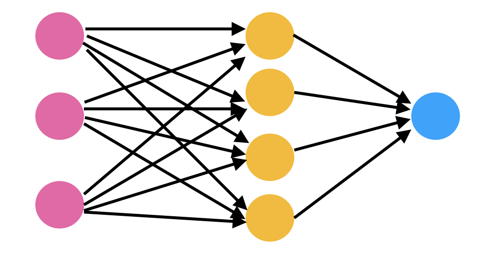
In the image above you can see a very casual diagram of a neural network. It has some colored circles connected to each other with arrows pointing to a particular direction. These colored circles are sometimes referred to as neurons.

These neurons are nothing but mathematical functions which, when given some input, generate an output. The output of neurons depends on the input and the parameters of the neurons. We can update these parameters to get a desired value out of the network.

Each of these neurons are defined using sigmoid function. A sigmoid function gives an output between zero to one for every input it gets. These sigmoid units are connected to each other to form a neural network.

By connection here we mean that the output of one layer of sigmoid units is given as input to each sigmoid unit of the next layer. In this way our neural network produces an output for any given input. The process continues until we have reached the final layer. The final layer generates its output.

This process of a neural network generating an output for a given input is Forward Propagation. Output of final layer is also called the prediction of the neural network. Later in this article we will discuss how we evaluate the predictions. These evaluations can be used to tell whether our neural network needs improvement or not.

Right after the final layer generates its output, we calculate the cost function. The cost function computes how far our neural network is from making its desired predictions. The value of the cost function shows the difference between the predicted value and the truth value.

Our objective here is to minimize the value of the cost function. The process of minimization of the cost function requires an algorithm which can update the values of the parameters in the network in such a way that the cost function achieves its minimum value.

Algorithms such as gradient descent and stochastic gradient descent are used to update the parameters of the neural network. These algorithms update the values of weights and biases of each layer in the network depending on how it will affect the minimization of cost function. The effect on the minimization of the cost function with respect to each of the weights and biases of each of the input neurons in the network is computed by backpropagation.

Code

So, we now know the main ideas behind the neural networks. Let us start implementing these ideas into code. We will start by importing all the required libraries.

import numpy as np
import matplotlib.pyplot as plt

As I mentioned we are not going to use any of the deep learning libraries. So, we will mostly use numpy for performing mathematical computations efficiently.

The first step in building our neural network will be to initialize the parameters. We need to initialize two parameters for each of the neurons in each layer: 1) Weight and 2) Bias.

These weights and biases are declared in vectorized form. That means that instead of initializing weights and biases for each individual neuron in every single layer, we will create a vector (or a matrix) for weights and another one for biases, for each layer.

These weights and bias vectors will be combined with the input to the layer. Then we will apply the sigmoid function over that combination and send that as the input to the next layer.

layer_dimsholds the dimensions of each layer. We will pass these dimensions of layers to the init_parmsfunction which will use them to initialize parameters. These parameters will be stored in a dictionary called params. So in the params dictionary **params[‘W1’]**will represent the weight matrix for layer 1.

def init_params(layer_dims):
    np.random.seed(3)
    params = {}
    L = len(layer_dims)

    for l in range(1, L):
        params['W'+str(l)] = np.random.randn(layer_dims[l], layer_dims[l-1])*0.01
        params['b'+str(l)] = np.zeros((layer_dims[l], 1))

    return params

Great! We have initialized the weights and biases and now we will define the sigmoid function. It will compute the value of the sigmoid function for any given value of Z and will also store this value as a cache. We will store cache values because we need them for implementing backpropagation. The Z here is the linear hypothesis.

Note that the sigmoid function falls under the class of activation functions in the neural network terminology. The job of an activation function is to shape the output of a neuron.

For example, the sigmoid function takes input with discrete values and gives a value which lies between zero and one. Its purpose is to convert the linear outputs to non-linear outputs. There are different types of activation functions that can be used for better performance but we will stick to sigmoid for the sake of simplicity.

# Z (linear hypothesis) - Z = W*X + b , 
# W - weight matrix, b- bias vector, X- Input 

def sigmoid(Z):
	A = 1/(1+np.exp(np.dot(-1, Z)))
    cache = (Z)

    return A, cache

Now, let’s start writing code for forward propagation. We have discussed earlier that forward propagation will take the values from the previous layer and give it as input to the next layer. The function below will take the training data and parameters as inputs and will generate output for one layer and then it will feed that output to the next layer and so on.

def forward_prop(X, params):

    A = X # input to first layer i.e. training data
    caches = []
    L = len(params)//2
    for l in range(1, L+1):
        A_prev = A

        # Linear Hypothesis
        Z = np.dot(params['W'+str(l)], A_prev) + params['b'+str(l)] 

        # Storing the linear cache
        linear_cache = (A_prev, params['W'+str(l)], params['b'+str(l)]) 

        # Applying sigmoid on linear hypothesis
        A, activation_cache = sigmoid(Z) 

         # storing the both linear and activation cache
        cache = (linear_cache, activation_cache)
        caches.append(cache)

    return A, caches

A_prev _i_s input to the first layer. We will loop through all the layers of the network and will compute the linear hypothesis. After that it will take the value of Z (linear hypothesis) and will give it to the sigmoid activation function. Cache values are stored along the way and are accumulated in caches. Finally, the function will return the value generated and the stored cache.

Let’s now define our cost function.

def cost_function(A, Y):
    m = Y.shape[1]

    cost = (-1/m)*(np.dot(np.log(A), Y.T) + np.dot(log(1-A), 1-Y.T)) 

    return cost

As the value of the cost function decreases, the performance of our model becomes better. The value of the cost function can be minimized by updating the values of the parameters of each of the layers in the neural network. Algorithms such as Gradient Descent are used to update these values in such a way that the cost function is minimized.

Gradient Descent updates the values with the help of some updating terms. These updating terms called gradients are calculated using the backpropagation. Gradient values are calculated for each neuron in the network and it represents the change in the final output with respect to the change in the parameters of that particular neuron.

def one_layer_backward(dA, cache):
    linear_cache, activation_cache = cache

    Z = activation_cache
    dZ = dA*sigmoid(Z)*(1-sigmoid(Z)) # The derivative of the sigmoid function

    A_prev, W, b = linear_cache
    m = A_prev.shape[1]

    dW = (1/m)*np.dot(dZ, A_prev.T)
    db = (1/m)*np.sum(dZ, axis=1, keepdims=True)
    dA_prev = np.dot(W.T, dZ)

    return dA_prev, dW, db

The code above runs the backpropagation step for one single layer. It calculates the gradient values for sigmoid units of one layer using the cache values we stored previously. In the activation cache we have stored the value of Z for that layer. Using this value we will calculate the dZ, which is the derivative of the cost function with respect to the linear output of the given neuron.

Once we have calculated all of that, we can calculate dW, db and dA_prev, which are the derivatives of cost function with respect the weights, biases and previous activation respectively. I have directly used the formulae in the code. If you are not familiar with calculus then it might seem too complicated at first. But for now think about it as any other math formula.

After that we will use this code to implement backpropagation for the entire neural network. The function backprop implements the code for that. Here, we have created a dictionary for mapping gradients to each layer. We will loop through the model in a backwards direction and compute the gradient.

def backprop(AL, Y, caches):
    grads = {}
    L = len(caches)
    m = AL.shape[1]
    Y = Y.reshape(AL.shape)

    dAL = -(np.divide(Y, AL) - np.divide(1-Y, 1-AL))

    current_cache = caches[L-1]
    grads['dA'+str(L-1)], grads['dW'+str(L-1)], grads['db'+str(L-1)] = one_layer_backward(dAL, current_cache)

    for l in reversed(range(L-1)):

        current_cache = caches[l]
        dA_prev_temp, dW_temp, db_temp = one_layer_backward(grads["dA" + str(l+1)], current_cache)
        grads["dA" + str(l)] = dA_prev_temp
        grads["dW" + str(l + 1)] = dW_temp
        grads["db" + str(l + 1)] = db_temp

    return grads

Once, we have looped through all the layers and computed the gradients, we will store those values in the grads dictionary and return it.

Finally, using these gradient values we will update the parameters for each layer. The function update_parameters goes through all the layers and updates the parameters and returns them.

def update_parameters(parameters, grads, learning_rate):
    L = len(parameters) // 2

    for l in range(L):
        parameters['W'+str(l+1)] = parameters['W'+str(l+1)] -learning_rate*grads['W'+str(l+1)]
        parameters['b'+str(l+1)] = parameters['b'+str(l+1)] -  learning_rate*grads['b'+str(l+1)]

    return parameters

Finally, it’s time to put it all together. We will create a function called train for training our neural network.

def train(X, Y, layer_dims, epochs, lr):
    params = init_params(layer_dims)
    cost_history = []

    for i in range(epochs):
        Y_hat, caches = forward_prop(X, params)
        cost = cost_function(Y_hat, Y)
        cost_history.append(cost)
        grads = backprop(Y_hat, Y, caches)

        params = update_parameters(params, grads, lr)

    return params, cost_history

This function will go through all the functions step by step for a given number of epochs. After finishing that, it will return the final updated parameters and the cost history. Cost history can be used to evaluate the performance of your network architecture.

Conclusion

If you are still reading this, Thanks! This article was a little complicated, so what I suggest you to do is to try playing around with the code. You might get some more insights out of it and maybe you might find some errors in the code too.

---

#python #machine-learning