I recently wrote an introductory article to geospatial visualizations in R, which quickly became my most read article by a factor of 5 (thanks, btw!). It was fantastic seeing how interested people were in geospatial data visualization, because at this point it’s become one of my favorite things on the planet.

That being said, I felt like I had left some cards on the table; for one, I hadn’t discussed ggplot2. Better yet, this second way was even prettier.

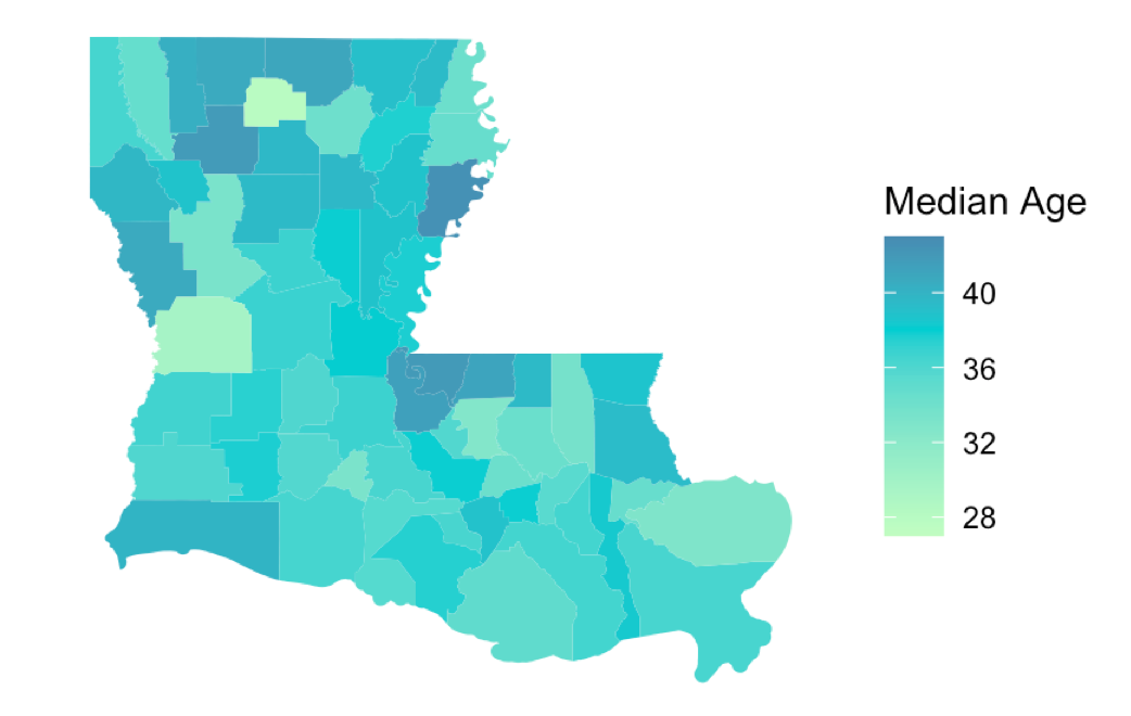
In this tutorial, we’re going to be using 2010 Census data to show off the wonders of graphing with R’s ggplot2 library. Just like last time, it’s only 3 steps —so grab some popcorn and let’s get started!

Step 1: Download 2010 Census Dataset

The simplest step ever; just go to my Github repo and download county_census.zip.

It’s a pretty big file; once it downloads, unzip it and you’re ready to go.

Step 2: Install Libraries & Upload Census Data to R

We’re going to be using 3 R libraries, which are maptools, rgdal, and ggplot2. We’re also going to run a command, readShapeSpatial(), which will prompt you for the file you want to use.

• Be sure to open County_2010Census_DP1.shpwhen prompted (this was downloaded in the previous step).

# Geospatial Visualization in R
	#~~~~~~~~~~~~~~~~~~~~~~~~~~~~~~~~~~~~~~~~~~~~~~~~~~
	rm(list=ls())
	install.packages(c("maptools", 
	                   "rgdal",
	                   "ggplot2"))

	library(maptools)
	library(rgdal)
	library(ggplot2)

	# unzip county_census file 
	# run this command and navigate to County_2010Census_DP1.shp when prompted 
	counties <- readShapeSpatial(file.choose(), proj4string = CRS("+proj=longlat +datum=WGS84"))
	#~~~~~~~~~~~~~~~~~~~~~~~~~~~~~~~~~~~~~~~~~~~~~~~~~~

#ggplot2 #data-science #programming #geospatial #visualization