Deep Learning and Neural Networks with Python and Pytorch p.1 - Introduction
Hello and welcome to a deep learning with Python and Pytorch tutorial series. It’s been a while since I last did a full coverage of deep learning on a lower level, and quite a few things have changed both in the field and regarding my understanding of deep learning.
For this series, I am going to be using Pytorch as our deep learning framework, though later on in the series we will also build a neural network from scratch.
I also have a tutorial miniseries for machine learning with Tensorflow and Keras if you’re looking for TensorFlow specifically.
Once you know one framework and how neural networks work, you should be able to move freely between the other frameworks quite easily.
What are neural networks?
I am going to assume many people are starting fresh, so I will quickly explain neural networks. It’s my belief that you’re going to learn the most by actually working with this technology, so I will be brief, but it can be useful to have a basic understanding going in.
Neural networks at their core are just another tool in the set of machine learning algorithms.
Neural networks consist of a bunch of “neurons” which are values that start off as your input data, and then get multiplied by weights, summed together, and then passed through an activation function to produce new values, and this process then repeats over however many “layers” your neural network has to then produce an output.
It looks something like
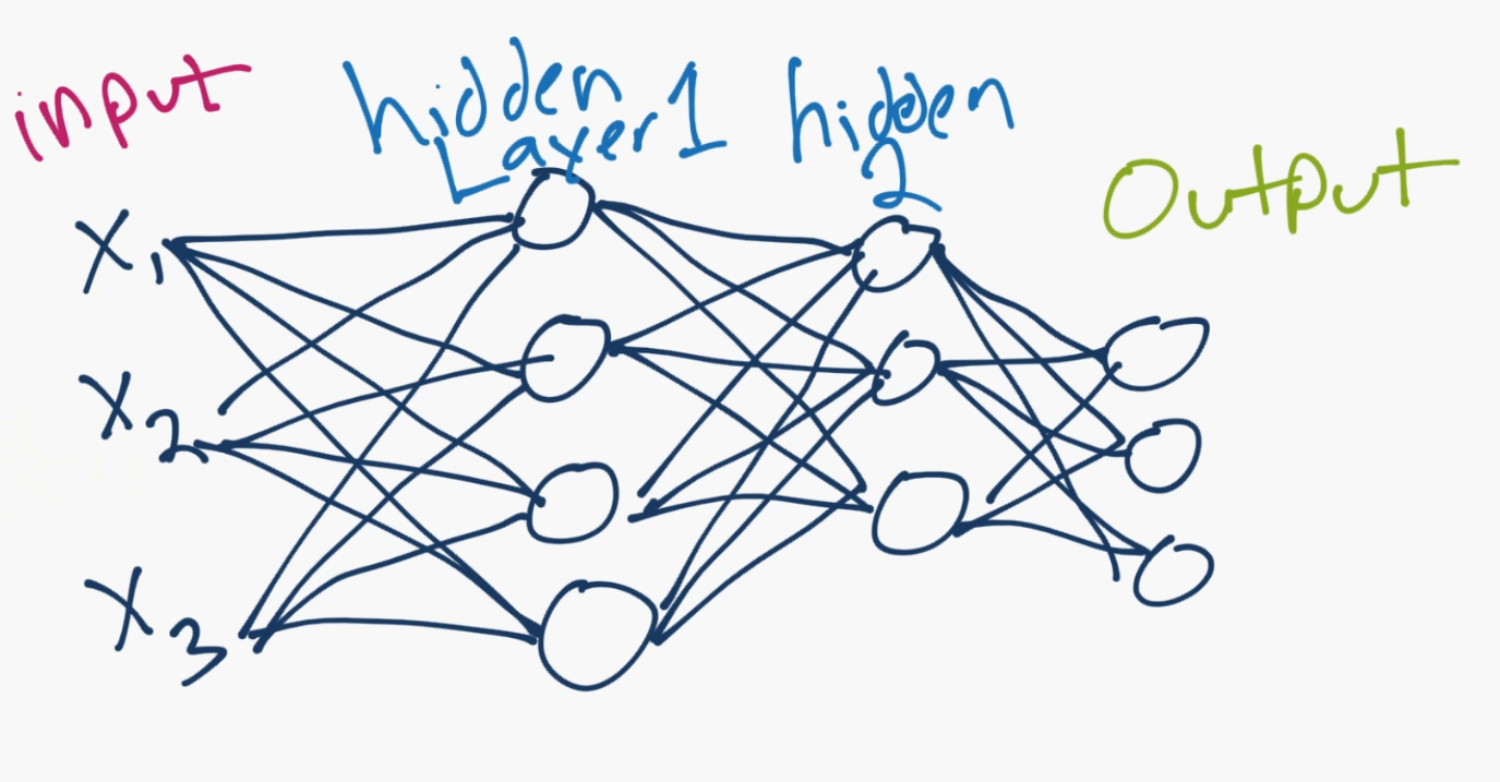
The X1, X2, X3 are the “features” of your data. These could be pixel values of an image, or some other numerical characteristic that describes your data.
In your hidden layers (“hidden” just generally refers to the fact that the programmer doesn’t really set or control the values to these layers, the machine does), these are neurons, numbering in however many you want (you control how many there are, just not the value of those neurons), and then they lead to an output layer. The output is usually either a single neuron for regression tasks, or as many neurons as you have classes. In the above case, there are 3 output neurons, so maybe this neural network is classifying dogs vs cats vs humans. Each neuron’s value can be thought of as a confidence score for if the neural network thinks it’s that class.
Whichever neuron has the highest value, that’s the predicted class! So maybe the top of the three output neurons is “human,” then “dog” in the middle and then “cat” on the bottom. If the human value is the largest one, then that would be the prediction of the neural network.
Connecting all of the neurons are those lines. Each of them is a weight, and possibly a bias. So the inputs get multiplied by the weights, the biases are added in, then it gets summed at the next neuron, passed through an activation function, to be the next input value for the next one!
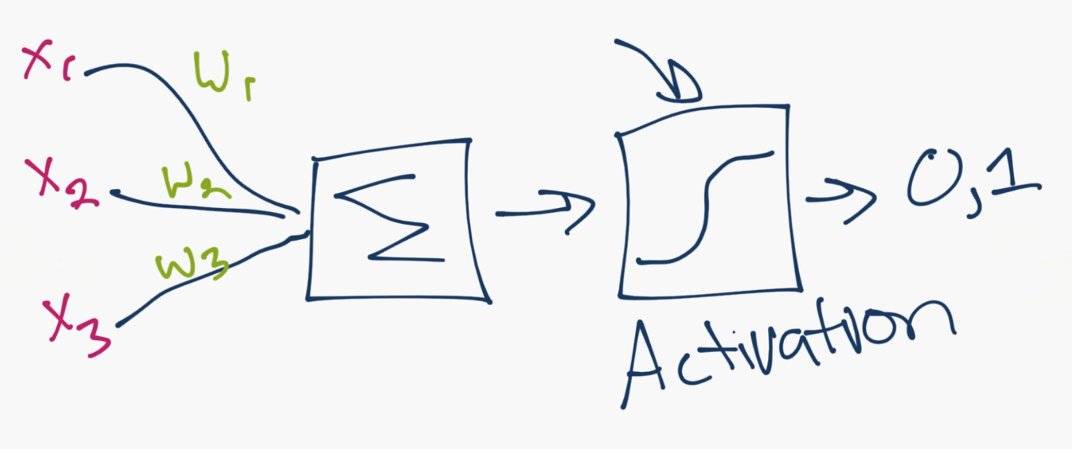
Above is an example of this “zoomed in” so to speak to show the mechanism for just a single neuron. You can see the inputs from other neurons come in, they’re multiplied by the weights, then they are summed together. After this summation, they pass through an activation function. The activation function’s job is to calculate whether or not, or how much, a neuron is “firing.” A neuron could output a 0 or 1 to be off or on, but also, more commonly, could instead output a range between 0 and 1, for example, which serves as input to the next layer.
How does a neural network “learn?”
For now, we’ll just consider the “supervised learning” approach, where the programmer shows the neural network the input data, and then also tells the machine what the output should be.
It then becomes the machine’s job to figure out how to adjust the weights (every line is a weight) such that the output of the model is as close as possible to the classifications that the programmer tells the machine that everything is. The machine aims to do this not just for a single sample, but for up to millions, or more of samples! …hunting by slowly tweaking weights, like turning and tweaking nobs in the system, in such a way so as to get closer and closer to the target/desired output.
Alright, you’re basically an expert now. Let’s get to Pytorch. If you’re still confused about certain things, that’s totally fine. Most, if not all, should be ironed out by actually working with this stuff. If you are confused at any point, however, just come to the discord channel: discord.gg/sentdex and ask your question in one of the help channels.
What you will need for this series:
- Python 3+. I will be using Python 3.7 specifically.
- Pytorch. I am using version 1.2.0 here.
- Understanding of the Python 3 basics
- Understanding of OOP and other intermediate concepts
Optionally, you may want to be running things on a GPU, rather than your CPU.
Why GPU?
We often want to run on the GPU because the thing we do with these tensor-processing libraries is we compute huge numbers of simple calculations. Each “core” of your CPU can only do 1 thing. With virtual cores, this doubles, but CPUs were meant to work on much more complicated, hard-to-solve, problems at a time. GPUs were intended to help generate graphics, which also require many small/simple calculations. As such, your CPU probably does somewhere between 8 and 24 calculations at a time. A decent GPU will do thousands.
For this tutorial, you can still follow along on your CPU, and probably any CPU will work. For just about any practical use-case of deep learning,however, you really are going to need a good GPU.
Cloud GPUs
There are some “free” platforms that do offer GPUs on a free tier, but, again, this wont be practical for any real case, and eventually you will want to upgrade your account there and then you will be paying prices typically above industry standard for what you’re getting. There are no corners to cut, at some point, you’re going to want a high-ish end GPU locally, or in the cloud.
Currently, in the cloud, the best bang for your buck option is Linode.com. I have a tutorial on how to efficiently make use of your cloud GPU as well, which uses Linode.
1.50 USD an hour can still be cost prohibitive, however, and many tasks wont need this kind of power. For the next best option, there is Paperspace, which offers cheaper GPUs and is super simple to setup. Here, you can get a deep-learning viable GPU for $0.50/hr, and you only pay while your machine is turned on.
Local GPUs
If you want to use your own GPU locally and you’re on Linux, Linode has a good Cuda Toolkit and CuDNN setup tutorial.
If you’re on Windows, then just get Cuda Toolkit 10.0.
Next, download CuDNN for Cuda Toolkit 10.0 (you may need to create an account and be logged in for this step).
Install the CUDA Toolkit, then extract the CuDNN files. From those CuDNN files (the dirs bin, include, and lib), you just need to move them to your Cuda Toolkit location, which is likely: C:\Program Files\NVIDIA GPU Computing Toolkit\CUDA\v10.0, which should also have bin, include, and lib dirs which you will merge with.
If you’re having a hard time with this, come to Discord.gg/sentdex and we’ll help to get you setup!
…or you can just stick with the CPU version of things!
What is Pytorch?
The Pytorch library, like the other deep learning libraries, really is just a library that does operations on tensors.
What’s a tensor?!
You can just think of a tensor like an array. Really all we’re doing is basically multiplying arrays here. That’s all there is to it. The fancy bits are when we run an optimization algorithm on all those weights to start modifying them. Neural networks themselves are actually super basic and simple. Their optimization is a little more challenging, but most of these deep learning libraries also help you a bit with that math. If you want to learn how to do everything yourself by hand, stay tuned later in the series. I just don’t think it would be wise to lead with that.
So, let’s poke with some tensors.
import torch

x = torch.Tensor([5,3])
y = torch.Tensor([2,1])

print(x*y)
tensor([10.,  3.])
So yeah, it’s just [5 2, 3 1]. Simple stuff!
Because it’s a lot of operations on arrays, Pytorch aims to mimic the very popular numeric library in Python called NumPy. Many of the exact same methods exist, usually with the same names, but sometimes different ones. One common task is to make an “empty” array, of some shape. In NumPy, we use np.zeros. In Pytorch, we do the same!
x = torch.zeros([2,5])
print(x)
tensor([[0., 0., 0., 0., 0.],
        [0., 0., 0., 0., 0.]])
print(x.shape)
torch.Size([2, 5])
If you need to generate an array of random values, but a specific shape
y = torch.rand([2,5])
print(y)
tensor([[0.2632, 0.9136, 0.5702, 0.9915, 0.4885],
        [0.5025, 0.7631, 0.5265, 0.4594, 0.1881]])
And no, I am not wasting your time with any of these examples. We will be using all of these methods, and learning more along the way.
For the last one, how about a reshape? It turns out Pytorch decided to come up with a new name that no one else uses, they call it .view()
For people coming here from Numpy or other ML libraries, that’ll be a goofy one, but pretty quick to remember.
So, in the above, we have 2 tensors, with 5 values in each. We could flatten this to be 1 tensor with 10 values. To do this, we would use .view():
y.view([1,10])
tensor([[0.2632, 0.9136, 0.5702, 0.9915, 0.4885, 0.5025, 0.7631, 0.5265, 0.4594,
         0.1881]])
I don’t totally mind this naming convention. You’re literally “viewing” that tensor as a 1x10 now. It doesn’t actually modify the tensor:
y
tensor([[0.2632, 0.9136, 0.5702, 0.9915, 0.4885],
        [0.5025, 0.7631, 0.5265, 0.4594, 0.1881]])
Of course you can re-assign:
y = y.view([1,10])
y
tensor([[0.2632, 0.9136, 0.5702, 0.9915, 0.4885, 0.5025, 0.7631, 0.5265, 0.4594,
         0.1881]])
Alright, there’s your super fast introduction to Pytorch and neural networks. In the next tutorial, we’ll be working on the input to our neural network, the data.
One of the very few things that we have control over when it comes to neural networks is the data, and the format/structure of this data.
First we have to acquire that data, then we have to consider how to convert the data to numerical values, consider things like scaling, and then figure out how we will be showing this data to the neural network.
Deep Learning and Neural Networks with Python and Pytorch p.2 - Data
So now that you know the basics of what Pytorch is, let’s apply it using a basic neural network example. The very first thing we have to consider is our data.
#### Neural Network InputSo now that you know the basics of what Pytorch is, let’s apply it using a basic neural network example. The very first thing we have to consider is our data. In most tutorials, this bit is often overlooked in the interest of going straight to the training of a neural network. That said, as a programmer working with neural networks, one of your largest tasks is preprocessing your data and formatting it in such as way to be easiest for the neural network to work with.
First, we need a dataset.
We’re just going to use data from Pytorch’s “torchvision.” Pytorch has a relatively handy inclusion of a bunch of different datasets, including many for vision tasks, which is what torchvision is for.
We’re going to first start off by using Torchvision because you should know it exists, plus it alleviates us the headache of dealing with datasets from scratch.
That said, this is the probably the last time that we’re going to do it this way. While it’s nice to load and play with premade datasets, it’s very rare that we get to do that in the real world, so it is essential that we learn how to start from a more raw dataset.
For now though, we’re just trying to learn about how to do a basic neural network in pytorch, so we’ll use torchvision here, to load the MNIST dataset, which is a image-based dataset showing handwritten digits from 0-9, and your job is to write a neural network to classify them.
To begin, let’s make our imports and load in the data:
import torch
import torchvision
from torchvision import transforms, datasets

train = datasets.MNIST('', train=True, download=True,
                       transform=transforms.Compose([
                           transforms.ToTensor()
                       ]))

test = datasets.MNIST('', train=False, download=True,
                       transform=transforms.Compose([
                           transforms.ToTensor()
                       ]))
Above, we’re just loading in the dataset, shuffling it, and applying any transforms/pre-processing to it.
Next, we need to handle for how we’re going to iterate over that dataset:
trainset = torch.utils.data.DataLoader(train, batch_size=10, shuffle=True)
testset = torch.utils.data.DataLoader(test, batch_size=10, shuffle=False)
You’ll see later why this torchvision stuff is basically cheating! For now though, what have we done? Well, quite a bit.
Training and Testing data split
To train any machine learning model, we want to first off have training and validation datasets. This is so we can use data that the machine has never seen before to “test” the machine.
Shuffling
Then, within our training dataset, we generally want to randomly shuffle the input data as much as possible to hopefully not have any patterns in the data that might throw the machine off.
For example, if you fed the machine a bunch of images of zeros, the machine would learn to classify everything as zero. Then you’d start feeding it ones, and the machine would figure out pretty quick to classify everything as ones…and so on. Whenever you stop, the machine would probably just classify everything as the last thing you trained on. If you shuffle the data, your machine is much more likely to figure out what’s what.
Scaling and normalization
Another consideration at some point in the pipeline is usually scaling/normalization of the dataset. In general, we want all input data to be between zero and one. Often many datasets will contain data in ranges that are not within this range, and we generally will want to come up with a way to scale the data to be within this range.
For example, an image is comprised of pixel values, most often in the range of 0 to 255. To scale image data, you usually just divide by 255. That’s it. Even though all features are just pixels, and all you do is divide by 255 before passing to the neural network, this makes a huge difference.
Batches
Once you’ve done all this, you then want to pass your training dataset to your neural network.
Not so fast!
There are two major reasons why you can’t just go and pass your entire dataset at once to your neural network:
- Neural networks shine and outperform other machine learning techniques because of how well they work on big datasets. Gigabytes. Terabytes. Petabytes! When we’re just learning, we tend to play with datasets smaller than a gigabyte, and we can often just toss the entire thing into the VRAM of our GPU or even more likely into RAM.
Unfortunately, in practice, you would likely not get away with this.
- The aim with neural networks is to have the network generalize with the data. We want the neural network to actually learn general principles. That said, neural networks often have millions, or tens of millions, of parameters that they can tweak to do this. This means neural networks can also just memorize things. While we hope neural networks will generalize, they often learn to just memorize the input data. Our job as the scientist is to make it as hard as possible for the neural network to just memorize.
This is another reason why we often track “in sample” validation acccuracy and “out of sample” validation accuracy. If these two numbers are similar, this is good. As they start to diverge (in sample usually goes up considerably while out of sample stays the same or drops), this usually means your neural network is starting to just memorize things.
One way we can help the neural network to not memorize is, at any given time, we feed only some specific batch size of data. This is often something between 8 and 64.
Although there is no actual reason for it, it’s a common trend in neural networks to use base 8 numbers for things like neuron counts, batch sizes…etc.
This batching helps because, with each batch, the neural network does a back propagation for new, updated weights with hopes of decreasing that loss.
With one giant passing of your data, this would include neuron changes that had nothing to do with general principles and were just brute forcing the operation.
By passing many batches, each with their own gradient calcs, loss, and backprop, this means each time the neural network optimizes things, it will sort of “keep” the changes that were actually useful, and erode the ones that were just basically memorizing the input data.
Given a large enough neural network, however, even with batches, your network can still just simply memorize.
This is also why we often try to make the smallest neural network as possible, so long as it still appears to be learning. In general, this will be a more successful model long term.
Now what?
Well, we have our data, but what is it really? How do we work with it? We can iterate over our data like so:
for data in trainset:
    print(data)
    break
[tensor([[[[0., 0., 0.,  ..., 0., 0., 0.],
          [0., 0., 0.,  ..., 0., 0., 0.],
          [0., 0., 0.,  ..., 0., 0., 0.],
          ...,
          [0., 0., 0.,  ..., 0., 0., 0.],
          [0., 0., 0.,  ..., 0., 0., 0.],
          [0., 0., 0.,  ..., 0., 0., 0.]]],

        [[[0., 0., 0.,  ..., 0., 0., 0.],
          [0., 0., 0.,  ..., 0., 0., 0.],
          [0., 0., 0.,  ..., 0., 0., 0.],
          ...,
          [0., 0., 0.,  ..., 0., 0., 0.],
          [0., 0., 0.,  ..., 0., 0., 0.],
          [0., 0., 0.,  ..., 0., 0., 0.]]],

        [[[0., 0., 0.,  ..., 0., 0., 0.],
          [0., 0., 0.,  ..., 0., 0., 0.],
          [0., 0., 0.,  ..., 0., 0., 0.],
          ...,
          [0., 0., 0.,  ..., 0., 0., 0.],
          [0., 0., 0.,  ..., 0., 0., 0.],
          [0., 0., 0.,  ..., 0., 0., 0.]]],

        ...,

        [[[0., 0., 0.,  ..., 0., 0., 0.],
          [0., 0., 0.,  ..., 0., 0., 0.],
          [0., 0., 0.,  ..., 0., 0., 0.],
          ...,
          [0., 0., 0.,  ..., 0., 0., 0.],
          [0., 0., 0.,  ..., 0., 0., 0.],
          [0., 0., 0.,  ..., 0., 0., 0.]]],

        [[[0., 0., 0.,  ..., 0., 0., 0.],
          [0., 0., 0.,  ..., 0., 0., 0.],
          [0., 0., 0.,  ..., 0., 0., 0.],
          ...,
          [0., 0., 0.,  ..., 0., 0., 0.],
          [0., 0., 0.,  ..., 0., 0., 0.],
          [0., 0., 0.,  ..., 0., 0., 0.]]],

        [[[0., 0., 0.,  ..., 0., 0., 0.],
          [0., 0., 0.,  ..., 0., 0., 0.],
          [0., 0., 0.,  ..., 0., 0., 0.],
          ...,
          [0., 0., 0.,  ..., 0., 0., 0.],
          [0., 0., 0.,  ..., 0., 0., 0.],
          [0., 0., 0.,  ..., 0., 0., 0.]]]]), tensor([2, 3, 1, 2, 0, 8, 9, 6, 1, 2])]
Each iteration will contain a batch of 10 elements (that was the batch size we chose), and 10 classes. Let’s just look at one:
X, y = data[0][0], data[1][0]
X is our input data. The features. The thing we want to predict. y is our label. The classification. The thing we hope the neural network can learn to predict. We can see this by doing.
data[0] is a bunch of features for things and data[1] is all the targets. So:
print(data[1])
tensor([2, 3, 1, 2, 0, 8, 9, 6, 1, 2])
As you can see, data[1] is just a bunch of labels. So, since data[1][0] is a 2, we can expect data[0][0] to be an image of a 2. Let’s see!
import matplotlib.pyplot as plt  ## pip install matplotlib

plt.imshow(data[0][0].view(28,28))
plt.show()

Clearly a 2 indeed.
So, for our checklist:
- We’ve got our data of various featuresets and their respective classes.
- That data is all numerical.
- We’ve shuffled the data.
- We’ve split the data into training and testing groups.
- Is the data scaled?
- Is the data balanced?
Looks like we have a couple more questions to answer. First off is it scaled? Remember earlier I warned that the neural network likes data to be scaled between 0 and 1 or -1 and 1. Raw imagery data is usually RGB, where each pixel is a tuple of values of 0-255, which is a problem. 0 to 255 is not scaled. How about our dataset here? Is it 0-255? or is it scaled already for us? Let’s check out some lines:
data[0][0][0][0]
tensor([0., 0., 0., 0., 0., 0., 0., 0., 0., 0., 0., 0., 0., 0., 0., 0., 0., 0., 0., 0., 0., 0., 0., 0.,
        0., 0., 0., 0.])
Hmm, it’s empty. Makes sense, the first few rows are blank probably in a lot of images. The 2 up above certainly is.
data[0][0][0][3]
tensor([0.0000, 0.0000, 0.0000, 0.0000, 0.0000, 0.0000, 0.0000, 0.0000, 0.0000,
        0.0000, 0.0118, 0.4157, 0.9059, 0.9961, 0.9216, 0.5647, 0.1882, 0.0000,
        0.0000, 0.0000, 0.0000, 0.0000, 0.0000, 0.0000, 0.0000, 0.0000, 0.0000,
        0.0000])
Ah okay, there we go, we can clearly see that… yep this image data is actually already scaled for us.
… in the real world, it wont be.
Like I said: Cheating! Hah. Alright. One more question: Is the data balanced?
What is data balancing?
Recall before how I explained that if we don’t shuffle our data, the machine will learn things like what the last few hundred classes were in a row, and probably just predict that from there on out.
Well, with data balancing, a similar thing could occur.
Imagine you have a dataset of cats and dogs. 7200 images are dogs, and 1800 are cats. This is quite the imbalance. The classifier is highly likely to find out that it can very quickly and easily get to a 72% accuracy by simple always predicting dog. It is highly unlikely that the model will recover from something like this.
Other times, the imbalance isn’t quite as severe, but still enough to make the model almost always predict a certain way except in the most obvious-to-it-of cases. Anyway, it’s best if we can balance the dataset.
By “balance,” I mean make sure there are the same number of examples for each classifications in training.
Sometimes, this simply isn’t possible. There are ways for us to handle for this with special class weighting for the optimizer to take note of, but, even this doesn’t always work. Personally, I’ve never had success with this in any real world application.
In our case, how might we confirm the balance of data? Well, we just need to iterate over everything and make a count. Pretty simple:
total = 0
counter_dict = {0:0, 1:0, 2:0, 3:0, 4:0, 5:0, 6:0, 7:0, 8:0, 9:0}

for data in trainset:
    Xs, ys = data
    for y in ys:
        counter_dict[int(y)] += 1
        total += 1

print(counter_dict)

for i in counter_dict:
    print(f"{i}: {counter_dict[i]/total*100.0}%")
{0: 5923, 1: 6742, 2: 5958, 3: 6131, 4: 5842, 5: 5421, 6: 5918, 7: 6265, 8: 5851, 9: 5949}
0: 9.871666666666666%
1: 11.236666666666666%
2: 9.93%
3: 10.218333333333334%
4: 9.736666666666666%
5: 9.035%
6: 9.863333333333333%
7: 10.441666666666666%
8: 9.751666666666667%
9: 9.915000000000001%
I am sure there’s a better way to do this, and there might be a built-in way to do it with torchvision. Anyway, as you can see, the lowest percentage is 9% and the highest is just over 11%. This should be just fine. We could balance this perfectly, but there’s likely no need for that.
I’d say we’re ready for passing it through a neural network, which is what we’ll be doing in the next tutorial.
Deep Learning and Neural Networks with Python and Pytorch p.3 - Building our Neural Network
In this tutorial, we’re going to focus on actually creating a neural network
Creating a Neural Network
In this tutorial, we’re going to focus on actually creating a neural network. In the previous tutorial, we went over the following code for getting our data setup:
import torch
import torchvision
from torchvision import transforms, datasets

train = datasets.MNIST('', train=True, download=True,
                       transform=transforms.Compose([
                           transforms.ToTensor()
                       ]))

test = datasets.MNIST('', train=False, download=True,
                       transform=transforms.Compose([
                           transforms.ToTensor()
                       ]))

trainset = torch.utils.data.DataLoader(train, batch_size=10, shuffle=True)
testset = torch.utils.data.DataLoader(test, batch_size=10, shuffle=False)
Now, let’s actually create our neural network model. To begin, we’re going to make a couple of imports from Pytorch:
import torch.nn as nn
import torch.nn.functional as F
The torch.nn import gives us access to some helpful neural network things, such as various neural network layer types (things like regular fully-connected layers, convolutional layers (for imagery), recurrent layers…etc). For now, we’ve only spoken about fully-connected layers, so we will just be using those for now.
The torch.nn.functional area specifically gives us access to some handy functions that we might not want to write ourselves. We will be using the relu or “rectified linear” activation function for our neurons. Instead of writing all of the code for these things, we can just import them, since these are things everyone will be needing in their deep learning code.
If you wish to learn about how to write those things, keep your eyes peeled for a neural network from scratch tutorial.
To make our model, we’re going to create a class. We’ll call this class net and this net will inhereit from the nn.Module class:
class Net(nn.Module):
    def __init__(self):
        super().__init__()

net = Net()
print(net)
Net()
Nothing much special here, but I know some people might be confused about the init method. Typically, when you inherit from a parent class, that init method doesn’t actually get run. This is how we can run that init method of the parent class, which can sometimes be required…because we actually want to initialize things! For example, let’s show some classes:
class a:
    '''Will be a parent class'''
    def __init__(self):
        print("initializing a")

class b(a):
    '''Inherits from a, but does not run a's init method '''
    def __init__(self):
        print("initializing b")

class c(a):
    '''Inhereits from a, but DOES run a's init method'''
    def __init__(self):
        super().__init__()
        print("initializing c")

b_ob = b()
initializing b
Notice how our b_ob doesn’t have the a class init method run. If we create a c_ob from the c class though:
c_ob = c()
initializing a
initializing c
Both init methods are run. Yay. Okay back to neural networks. Let’s define our layers
class Net(nn.Module):
    def __init__(self):
        super().__init__()
        self.fc1 = nn.Linear(28*28, 64)
        self.fc2 = nn.Linear(64, 64)
        self.fc3 = nn.Linear(64, 64)
        self.fc4 = nn.Linear(64, 10)

net = Net()
print(net)
All we’re doing is just defining values for some layers, we’re calling them fc1, fc2…etc, but you could call them whatever you wanted. The fc just stands for fully connected. Fully connected refers to the point that every neuron in this layer is going to be fully connected to attaching neurons. Nothing fancy going on here! Recall, each “connection” comes with weights and possibly biases, so each connection is a “parameter” for the neural network to play with.
In our case, we have 4 layers. Each of our nn.Linear layers expects the first parameter to be the input size, and the 2nd parameter is the output size.
So, our first layer takes in 28x28, because our images are 28x28 images of hand-drawn digits. A basic neural network is going to expect to have a flattened array, so not a 28x28, but instead a 1x784.
Then this outputs 64 connections. This means the next layer, fc2 takes in 64 (the next layer is always going to accept however many connections the previous layer outputs). From here, this layer ouputs 64, then fc3 just does the same thing.
fc4 takes in 64, but outputs 10. Why 10? Our “output” layer needs 10 neurons. Why 10 neurons? We have 10 classes.
Now, that’s great, we have those layers, but nothing really dictating how they interact with eachother, they’re just simply defined.
The simplest neural network is fully connected, and feed-forward, meaning we go from input to output. In one side and out the other in a “forward” manner. We do not have to do this, but, for this model, we will. So let’s define a new method for this network called forward and then dictate how our data will pass through this model:
class Net(nn.Module):
    def __init__(self):
        super().__init__()
        self.fc1 = nn.Linear(28*28, 64)
        self.fc2 = nn.Linear(64, 64)
        self.fc3 = nn.Linear(64, 64)
        self.fc4 = nn.Linear(64, 10)

    def forward(self, x):
        x = self.fc1(x)
        x = self.fc2(x)
        x = self.fc3(x)
        x = self.fc4(x)
        return x

net = Net()
print(net)
Net(
  (fc1): Linear(in_features=784, out_features=64, bias=True)
  (fc2): Linear(in_features=64, out_features=64, bias=True)
  (fc3): Linear(in_features=64, out_features=64, bias=True)
  (fc4): Linear(in_features=64, out_features=10, bias=True)
)
Notice the x is a parameter for the forward method. This will be our input data. As you can see, we literally just “pass” this data through the layers. This could in theory learn with some problems, but this is going to most likely cause some serious explosions in values. The neural network could control this, but probably wont. Instead, what we’re missing is an activation function for the layers.
Recall that we’re mimicking brain neurons that either are firing, or not. We use activation functions to take the sum of the input data * weights, and then to determine if the neuron is firing or not. Initially, these were often step functions that were literally either 0 or 1, but then we found that sigmoids and other types of functions were better.
Currently, the most popular is the rectified linear, or relu, activation function.
Basically, these activation functions are keeping our data scaled between 0 and 1.
Finally, for the output layer, we’re going to use softmax. Softmax makes sense to use for a multi-class problem, where each thing can only be one class or the other. This means the outputs themselves are a confidence score, adding up to 1.
class Net(nn.Module):
    def __init__(self):
        super().__init__()
        self.fc1 = nn.Linear(28*28, 64)
        self.fc2 = nn.Linear(64, 64)
        self.fc3 = nn.Linear(64, 64)
        self.fc4 = nn.Linear(64, 10)

    def forward(self, x):
        x = F.relu(self.fc1(x))
        x = F.relu(self.fc2(x))
        x = F.relu(self.fc3(x))
        x = self.fc4(x)
        return F.log_softmax(x, dim=1)

net = Net()
print(net)
Net(
  (fc1): Linear(in_features=784, out_features=64, bias=True)
  (fc2): Linear(in_features=64, out_features=64, bias=True)
  (fc3): Linear(in_features=64, out_features=64, bias=True)
  (fc4): Linear(in_features=64, out_features=10, bias=True)
)
At this point, we’ve got a neural network that we can actually pass data to, and it will give us an output. Let’s see. Let’s just create a random image:
X = torch.randn((28,28))
So this is like our images, a 28x28 tensor (array) of values ranging from 0 to 1. Our neural network wants this to be flattened, however so:
X = X.view(-1,28*28)
You should understand the 28*28 part, but why the leading -1?
Any input and output to our neural network is expected to be a group feature sets.
Even if you intend to just pass 1 set of features, you still have to pass it as a “list” of features.
In our case, we really just want a 1x784, and we could say that, but you will more often is -1 used in these shapings. Why? -1 suggests “any size”. So it could be 1, 12, 92, 15295…etc. It’s a handy way for that bit to be variable. In this case, the variable part is how many “samples” we’ll pass through.
output = net(X)
What should we be expecting the output to be? It should be a tensor that contains a tensor of our 10 possible classes:
output
tensor([[-2.3037, -2.2145, -2.3538, -2.3707, -2.1101, -2.4241, -2.4055, -2.2921,
         -2.2625, -2.3294]], grad_fn=<LogSoftmaxBackward>)
Great. Looks like the forward pass works and everything is as expected. Why was it a tensor in a tensor? Because input and output needs to be variable. Even if we just want to predict on one input, it needs to be a list of inputs and the output will be a list of outputs. Not really a list, it’s a tensor, but hopefully you understand what I mean.
Of course, those outputs are pretty worthless to us. Instead, we want to iterate over our dataset as well as do our backpropagation, which is what we’ll be getting into in the next tutorial.
Deep Learning and Neural Networks with Python and Pytorch p.4 - Training Model
In this deep learning with Python and Pytorch tutorial, we’ll be actually training this neural network by learning how to iterate over our data, pass to the model, calculate loss from the result, and then do backpropagation to slowly fit our model to the data.
Training our Neural Network
In the previous tutorial, we created the code for our neural network. In this deep learning with Python and Pytorch tutorial, we’ll be actually training this neural network by learning how to iterate over our data, pass to the model, calculate loss from the result, and then do backpropagation to slowly fit our model to the data.
Code up to this point:
import torch
import torchvision
from torchvision import transforms, datasets
import torch.nn as nn
import torch.nn.functional as F

train = datasets.MNIST('', train=True, download=True,
                       transform=transforms.Compose([
                           transforms.ToTensor()
                       ]))

test = datasets.MNIST('', train=False, download=True,
                       transform=transforms.Compose([
                           transforms.ToTensor()
                       ]))

trainset = torch.utils.data.DataLoader(train, batch_size=10, shuffle=True)
testset = torch.utils.data.DataLoader(test, batch_size=10, shuffle=False)

class Net(nn.Module):
    def __init__(self):
        super().__init__()
        self.fc1 = nn.Linear(28*28, 64)
        self.fc2 = nn.Linear(64, 64)
        self.fc3 = nn.Linear(64, 64)
        self.fc4 = nn.Linear(64, 10)

    def forward(self, x):
        x = F.relu(self.fc1(x))
        x = F.relu(self.fc2(x))
        x = F.relu(self.fc3(x))
        x = self.fc4(x)
        return F.log_softmax(x, dim=1)

net = Net()
print(net)
Net(
  (fc1): Linear(in_features=784, out_features=64, bias=True)
  (fc2): Linear(in_features=64, out_features=64, bias=True)
  (fc3): Linear(in_features=64, out_features=64, bias=True)
  (fc4): Linear(in_features=64, out_features=10, bias=True)
)
Luckily for us, the “data” that we’re using from Pytorch is actually nice fancy object that is making life easy for us at the moment. It’s already in pretty batches and we just need to iterate over it. Next, we want to calculate loss and specify our optimizer:
import torch.optim as optim

loss_function = nn.CrossEntropyLoss()
optimizer = optim.Adam(net.parameters(), lr=0.001)
Our loss_function is what calculates “how far off” our classifications are from reality. As humans, we tend to think of things in terms of either right, or wrong. With a neural network, and arguably humans too, our accuracy is actually some sort of scaling score.
For example, you might be highly confident that something is the case, but you are wrong. Compare this to a time when you really aren’t certain either way, but maybe think something, but are wrong. In these cases, the degree to which you’re wrong doesn’t matter in terms of the choice necessarily, but in terms of you learning, it does.
In terms of a machine learning by tweaking lots of little parameters to slowly get closer and closer to fitting, it definitely matters how wrong things are.
For this, we use loss, which is a measurement of how far off the neural network is from the targeted output. There are a few types of loss calculations. A popular one is mean squared error, but we’re trying to use these scalar-valued classes.
In general, you’re going to have two types of classes. One will just be a scalar value, the other is what’s called a one_hot array/vector.
In our case, a zero might be classified as:
0 or [1, 0, 0, 0, 0, 0, 0 ,0 ,0 ,0]
[1, 0, 0, 0, 0, 0, 0 ,0 ,0 ,0] is a one_hot array where quite literally one element only is a 1 and the rest are zero. The index that is hot is the classification.
A one_hot vector for a a 3 would be:
[0, 0, 0, 1, 0, 0, 0 ,0 ,0 ,0]
I tend to use one_hot, but this data is specifying a scalar class, so 0, or 1, or 2…and so on.
Depending on what your targets look like, you will need a specific loss.
For one_hot vectors, I tend to use mean squared error.
For these scalar classifications, I use cross entropy.
Next, we have our optimizer. This is the thing that adjusts our model’s adjustable parameters like the weights, to slowly, over time, fit our data. I am going to have us using Adam, which is Adaptive Momentum. This is the standard go-to optimizer usually. There’s a new one called rectified adam that is gaining steam. I haven’t had the chance yet to make use of that in any project, and I do not think it’s available as just an importable function in Pytorch yet, but keep your eyes peeled for it! For now, Adam will do just fine I’m sure. The other thing here is lr, which is the learning rate. A good number to start with here is 0.001 or 1e-3. The learning rate dictates the magnitude of changes that the optimizer can make at a time. Thus, the larger the LR, the quicker the model can learn, but also you might find that the steps you allow the optimizer to make are actually too big and the optimizer gets stuck bouncing around rather than improving. Too small, and the model can take much longer to learn as well as also possibly getting stuck.
Imagine the learning rate as the “size of steps” that the optimizer can take as it searches for the bottom of a mountain, where the path to the bottom isn’t necessarily a simple straight path down. Here’s some lovely imagery to help explain learning rate:
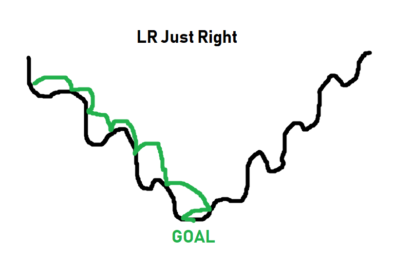
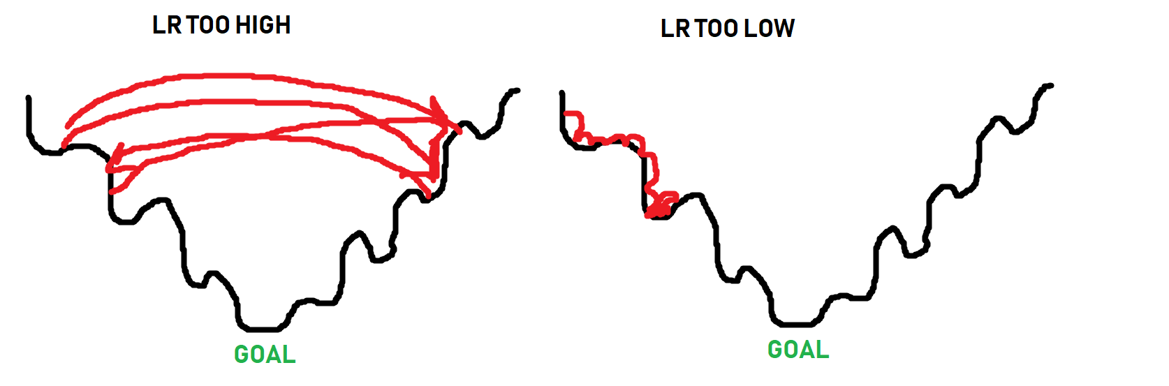 The black line is the “path” to the bottom of the optimization curve. When it comes to optimizing, sometimes you have to get worse in order to actually get beyond some local optimum. The optimizer doesn’t know what the absolute best spot could be, it just takes steps to see if it can find it. Thus, as you can see in the image, if the steps are too big, it will never get to the lower points. If the steps are too small (learning rate too small), it can get stuck as well long before it reaches a bottom. The goal is for something more like:
For simpler tasks, a learning rate of 0.001 usually is more than fine. For more complex tasks, you will see a learning rate with what’s called a decay. Basically you start the learning rate at something like 0.001, or 0.01…etc, and then over time, that learning rate gets smaller and smaller. The idea being you can initially train fast, and slowly take smaller steps, hopefully getthing the best of both worlds:
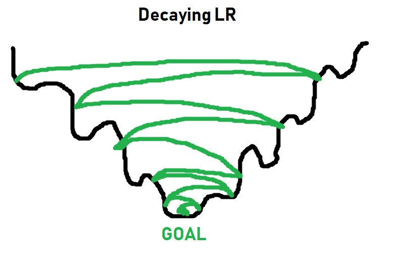
More on learning rates and decay later. For now, 0.001 will work just fine, and you just need to think of learning rate as what it sounds like: How quickly should we try to get this optimizer to optimize things.
Now we can iterate over our data. In general, you will make more than just 1 pass through your entire training dataset.
Each full pass through your dataset is referred to as an epoch. In general, you will probably have somewhere between 3 and 10 epochs, but there’s no hard rule here.
Too few epochs, and your model wont learn everything it could have.
Too many epochs and your model will over fit to your in-sample data (basically memorize the in-sample data, and perform poorly on out of sample data).
Let’s go with 3 epochs for now. So we will loop over epochs, and each epoch will loop over our data. Something like:
for epoch in range(3): ## 3 full passes over the data
    for data in trainset:  ## `data` is a batch of data
        X, y = data  ## X is the batch of features, y is the batch of targets.
        net.zero_grad()  ## sets gradients to 0 before loss calc. You will do this likely every step.
        output = net(X.view(-1,784))  ## pass in the reshaped batch (recall they are 28x28 atm)
        loss = F.nll_loss(output, y)  ## calc and grab the loss value
        loss.backward()  ## apply this loss backwards thru the network's parameters
        optimizer.step()  ## attempt to optimize weights to account for loss/gradients
    print(loss)  ## print loss. We hope loss (a measure of wrong-ness) declines!
tensor(0.4054, grad_fn=<NllLossBackward>)
tensor(0.4121, grad_fn=<NllLossBackward>)
tensor(0.0206, grad_fn=<NllLossBackward>)
Every line here is commented, but the concept of gradients might not be clear. Once we pass data through our neural network, getting an output, we can compare that output to the desired output. With this, we can compute the gradients for each parameter, which our optimizer (Adam, SGD…etc) uses as information for updating weights.
This is why it’s important to do a net.zero_grad() for every step, otherwise these gradients will add up for every pass, and then we’ll be re-optimizing for previous gradients that we already optimized for. There could be times when you intend to have the gradients sum per pass, like maybe you have a batch of 10, but you want to optimize per 50 or something. I don’t think people really do that, but the idea of Pytorch is to let you do whatever you want.
So, for each epoch, and for each batch in our dataset, what do we do?
- Grab the features (X) and labels (y) from current batch
- Zero the gradients (net.zero_grad)
- Pass the data through the network
- Calculate the loss
- Adjust weights in the network with the hopes of decreasing loss
As we iterate, we get loss, which is an important metric, but we care about accuracy. So, how did we do? To test this, all we need to do is iterate over our test set, measuring for correctness by comparing output to target values.
correct = 0
total = 0

with torch.no_grad():
    for data in testset:
        X, y = data
        output = net(X.view(-1,784))
        #print(output)
        for idx, i in enumerate(output):
            #print(torch.argmax(i), y[idx])
            if torch.argmax(i) == y[idx]:
                correct += 1
            total += 1

print("Accuracy: ", round(correct/total, 3))
Accuracy:  0.968
Yeah, I would say we did alright there.
import matplotlib.pyplot as plt

plt.imshow(X[0].view(28,28))
plt.show()

print(torch.argmax(net(X[0].view(-1,784))[0]))
tensor(7)
The above might be slightly confusing. I’ll break it down.
a_featureset = X[0]
reshaped_for_network = a_featureset.view(-1,784) ## 784 b/c 28*28 image resolution.
output = net(reshaped_for_network) #output will be a list of network predictions.
first_pred = output[0]
print(first_pred)
tensor([-1.9319e+01, -1.1778e+01, -1.0212e+01, -7.2939e+00, -1.8264e+01,
        -1.3537e+01, -3.7725e+01, -7.3906e-04, -1.1903e+01, -1.1936e+01],
       grad_fn=<SelectBackward>)
Which index value is the greatest? We use argmax to find this:
biggest_index = torch.argmax(first_pred)
print(biggest_index)
tensor(7)
There’s so much more we could do here with this example, but I think it’s best we move on.
More things to consider: Tracking/graphing loss and accuracy over time, comparing in and out of sample accuracy, maybe hand-drawing our own example to see if it works…etc.
As fun and easy as it is to use a pre-made dataset, one of the first things you really want to do once you learn deep learning is actually do something you’re interested in, which often means your own dataset that isn’t prepared for us like this one was.
In the coming tutorials, we’re going to discuss the convolutional neural network and classify images of dogs and cats, starting from the raw images, as well as covering some of the other topics like tracking training over time.
Deep Learning and Neural Networks with Python and Pytorch p.5 - Convnet Intro
Now that we’ve learned about the basic feed forward, fully connected, neural network, it’s time to cover a new one: the convolutional neural network, often referred to as a convnet or cnn.
Convolutional neural networks got their start by working with imagery.
Convolutional Neural Networks with Pytorch
Now that we’ve learned about the basic feed forward, fully connected, neural network, it’s time to cover a new one: the convolutional neural network, often referred to as a convnet or cnn.
Convolutional neural networks got their start by working with imagery. The idea of doing image analysis is to recognize things like objects, such as humans, or cars.
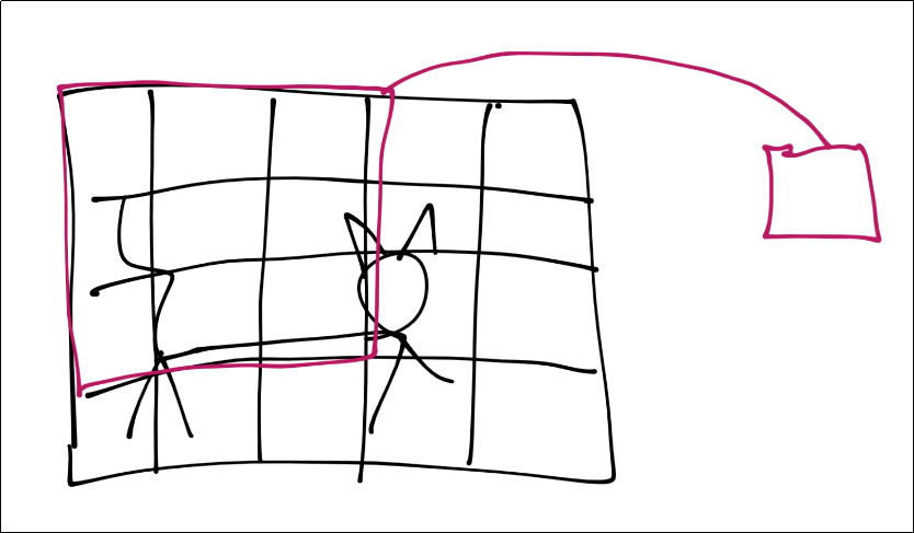
In order to recognize a car or a human, it’s fairly challenging to do so if you’re thinking of things 1 pixel at a time. Instead, a convolutional neural network aims to use a sliding window (a kernel) that takes into account a group of pixels, to hopefully recognize small features like “edges” or “curves” and then another layer might take combinations of edges or curves to detect shapes like squares or circles, or other complex types of shapes…and so on.
I will illustrate this process, starting with a picture of a cat

Next, let’s simulate a conversion to pixels
![]()
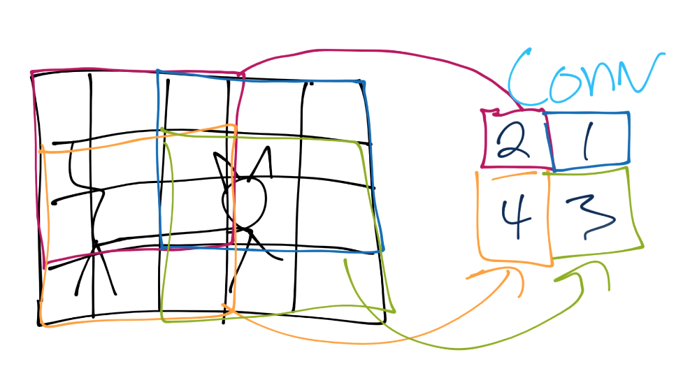
For the purposes of this tutorial, assume each square is a pixel. Next, for the convolution step, we’re going to take some n-sized window:
Those features are then condensed down into a single feature in a new featuremap.
Next, we slide that window over and repeat until with have a new set of featuremaps.
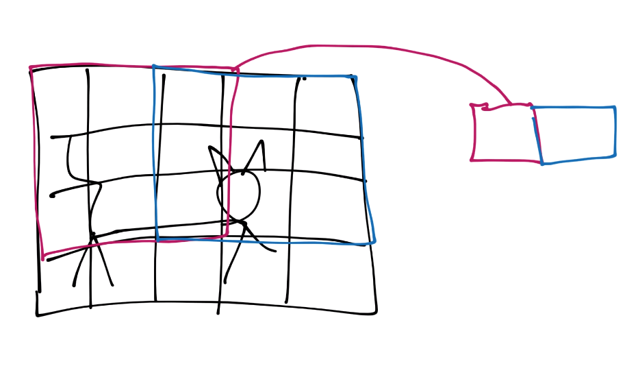
You continue this process until you’ve covered the entire image.
From here, we do pooling. Let’s say our convolution gave us (I forgot to put a number in the 2nd row’s most right square, assume it’s a 3 or less):
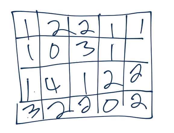
Now we’ll take a 3x3 pooling window:
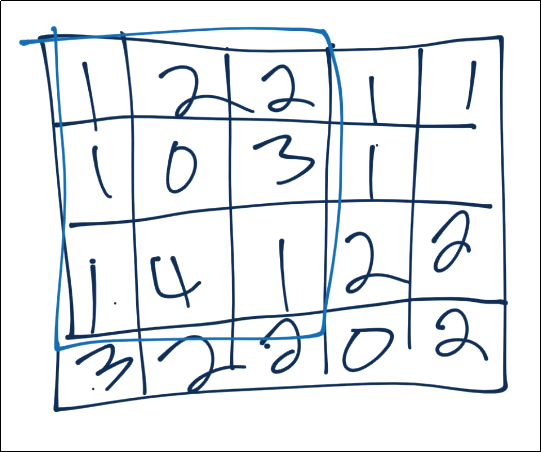
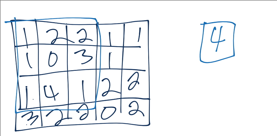
The most common form of pooling is “max pooling,” where we simple take the maximum value in the window, and that becomes the new value for that region.
We continue this process, until we’ve pooled, and have something like:
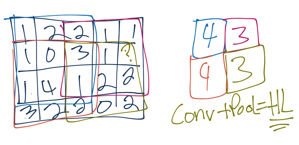
Often, after convolutional layers, we’ll have 1 or a few fully connected layers, and then the output. You could go straight from the final pooling to an output layer, however.
So, at their core, convnets are hunting first for low level types of features like lines and curves, then they look for combinations of those, and so on, to better understand what they’re looking at.
Let’s try our hands at a convnet example.
Getting data
To begin, we need a dataset.
I am going to have us use the Cats vs Dogs dataset.
This dataset consists of a bunch of images of cats and dogs. Different breeds, ages, sizes (both the animal and the image)…etc.
Once you have downloaded the dataset, you need to extract it. I would just extract it to the directory that you’re working in.
Preparing data
Rember how before I said using torchvision was cheating? Well it was, and now we have to build this data ourselves! To begin, let’s make sure you have all of the required libraries:
pip install opencv-python numpy tqdm matplotlib
Let’s make some imports:
import os
import cv2
import numpy as np
from tqdm import tqdm
Now to begin our data processing class:
class DogsVSCats():
    IMG_SIZE = 50
    CATS = "PetImages/Cat"
    DOGS = "PetImages/Dog"
    TESTING = "PetImages/Testing"
    LABELS = {CATS: 0, DOGS: 1}
    training_data = []
The IMG_SIZE is whatever we want, but we have to pick something. The images in the training data are all varying sizes and shapes. We’re going to normalize all of the images by reshaping them to all be the same size. I will go with 50x50.
Next are just some variables that hold where the directories with the data are. Once extracted, you wind up with 2 directories. One is Cat, the other is Dog and those contain a bunch of images.
We want to iterate through these two directories, grab the images, resize, scale, convert the class to number (cats = 0, dogs = 1), and add them to our training_data.
Continuing along in our class, let’s make a new method called make_training_data:
class DogsVSCats():
    IMG_SIZE = 50
    CATS = "PetImages/Cat"
    DOGS = "PetImages/Dog"
    TESTING = "PetImages/Testing"
    LABELS = {CATS: 0, DOGS: 1}
    training_data = []

    def make_training_data(self):
        for label in self.LABELS:
            for f in tqdm(os.listdir(label)):
                if "jpg" in f:
                    try:
                        pass
                    except Exception as e:
                        pass
                        #print(label, f, str(e))
All we’re doing so far is iterating through the cats and dogs directories, and looking through all of the images. Now let’s actually write the code to handle for the images:
class DogsVSCats():
    IMG_SIZE = 50
    CATS = "PetImages/Cat"
    DOGS = "PetImages/Dog"
    TESTING = "PetImages/Testing"
    LABELS = {CATS: 0, DOGS: 1}
    training_data = []

    def make_training_data(self):
        for label in self.LABELS:
            for f in tqdm(os.listdir(label)):
                if "jpg" in f:
                    try:
                        path = os.path.join(label, f)
                        img = cv2.imread(path, cv2.IMREAD_GRAYSCALE)
                        img = cv2.resize(img, (self.IMG_SIZE, self.IMG_SIZE))
                        self.training_data.append([np.array(img), np.eye(2)[self.LABELS[label]]])  ## do something like print(np.eye(2)[1]), just makes one_hot
                        #print(np.eye(2)[self.LABELS[label]])
                    except Exception as e:
                        pass
                        #print(label, f, str(e))
We read in the data, convert to grayscale, resize the image to whatever we chose, and then append the image data along with the associated class in number form to our training_data. Some images can’t be read, so we just pass on the exception. If you’re creating no data at all, then go ahead and print out the error, but it’s enough images to be annoying if I print out the error every time.
Once we have the data, is there anything we’ve not done to the data yet?
We want to check for balance, and we want to shuffle it. We can just use a counter again to see balance:
                        if label == self.CATS:
                            self.catcount += 1
                        elif label == self.DOGS:
                            self.dogcount += 1
Then we can just shuffle the training_data list at the end with
np.random.shuffle(self.training_data)
This process can take a while, longer than we’d like if we’re just tinkering with different values for our neural network. It’d be nice to just save where we are now after pre-processing, so we’ll also add a np.save.
Finally, I would just recommend using some sort of flag or something for if/when you change something like image shape or something like that, so you can easily re-run this code when needed.
Now our full code is:
REBUILD_DATA = True ## set to true to one once, then back to false unless you want to change something in your training data.

class DogsVSCats():
    IMG_SIZE = 50
    CATS = "PetImages/Cat"
    DOGS = "PetImages/Dog"
    TESTING = "PetImages/Testing"
    LABELS = {CATS: 0, DOGS: 1}
    training_data = []

    catcount = 0
    dogcount = 0

    def make_training_data(self):
        for label in self.LABELS:
            print(label)
            for f in tqdm(os.listdir(label)):
                if "jpg" in f:
                    try:
                        path = os.path.join(label, f)
                        img = cv2.imread(path, cv2.IMREAD_GRAYSCALE)
                        img = cv2.resize(img, (self.IMG_SIZE, self.IMG_SIZE))
                        self.training_data.append([np.array(img), np.eye(2)[self.LABELS[label]]])  ## do something like print(np.eye(2)[1]), just makes one_hot
                        #print(np.eye(2)[self.LABELS[label]])

                        if label == self.CATS:
                            self.catcount += 1
                        elif label == self.DOGS:
                            self.dogcount += 1

                    except Exception as e:
                        pass
                        #print(label, f, str(e))

        np.random.shuffle(self.training_data)
        np.save("training_data.npy", self.training_data)
        print('Cats:',dogsvcats.catcount)
        print('Dogs:',dogsvcats.dogcount)

if REBUILD_DATA:
    dogsvcats = DogsVSCats()
    dogsvcats.make_training_data()
PetImages/Cat
100%|a-^a-^a-^a-^a-^a-^a-^a-^a-^a-^a-^a-^a-^a-^a-^a-^a-^a-^a-^a-^a-^a-^a-^a-^a-^a-^a-^a-^a-^a-^a-^a-^a-^a-^a-^a-^a-^a-^a-^a-^a-^a-^a-^a-^| 12501/12501 [00:13<00:00, 918.70it/s]
PetImages/Dog
100%|a-^a-^a-^a-^a-^a-^a-^a-^a-^a-^a-^a-^a-^a-^a-^a-^a-^a-^a-^a-^a-^a-^a-^a-^a-^a-^a-^a-^a-^a-^a-^a-^a-^a-^a-^a-^a-^a-^a-^a-^a-^a-^a-^a-^| 12501/12501 [00:14<00:00, 862.58it/s]
Cats: 12476
Dogs: 12470
After you’ve built the data once, you should have the training_data.npy file. To use that, we just need to do:
training_data = np.load("training_data.npy", allow_pickle=True)
print(len(training_data))
24946
Now we can split our training data into X and y, as well as convert it to a tensor:
import torch

X = torch.Tensor([i[0] for i in training_data]).view(-1,50,50)
X = X/255.0
y = torch.Tensor([i[1] for i in training_data])
Now let’s take a peak at one of our samples:
import matplotlib.pyplot as plt

plt.imshow(X[0], cmap="gray")
<matplotlib.image.AxesImage at 0x1d58853ec50>
print(y[0])
tensor([1., 0.])
Alright! So now we have our training data in the form of inputs and outputs.
We still will eventually need to, for example, split this out into training/validation data, but the next thing we want to do is build our network. That’s what we’ll be doing in the next tutorial.
Deep Learning and Neural Networks with Python and Pytorch p.6 - Training Convnet
Welcome to part 6 of the deep learning with Python and Pytorch tutorials. Leading up to this tutorial, we’ve covered how to make a basic neural network, and now we’re going to cover how to make a slightly more complex neural network: The convolutional neural network, or Convnet/CNN.
Creating a Convolutional Neural Network in Pytorch
Welcome to part 6 of the deep learning with Python and Pytorch tutorials. Leading up to this tutorial, we’ve covered how to make a basic neural network, and now we’re going to cover how to make a slightly more complex neural network: The convolutional neural network, or Convnet/CNN.
Code up to this point:
import os
import cv2
import numpy as np
from tqdm import tqdm

REBUILD_DATA = False ## set to true to one once, then back to false unless you want to change something in your training data.

class DogsVSCats():
    IMG_SIZE = 50
    CATS = "PetImages/Cat"
    DOGS = "PetImages/Dog"
    TESTING = "PetImages/Testing"
    LABELS = {CATS: 0, DOGS: 1}
    training_data = []

    catcount = 0
    dogcount = 0

    def make_training_data(self):
        for label in self.LABELS:
            print(label)
            for f in tqdm(os.listdir(label)):
                if "jpg" in f:
                    try:
                        path = os.path.join(label, f)
                        img = cv2.imread(path, cv2.IMREAD_GRAYSCALE)
                        img = cv2.resize(img, (self.IMG_SIZE, self.IMG_SIZE))
                        self.training_data.append([np.array(img), np.eye(2)[self.LABELS[label]]])  ## do something like print(np.eye(2)[1]), just makes one_hot
                        #print(np.eye(2)[self.LABELS[label]])

                        if label == self.CATS:
                            self.catcount += 1
                        elif label == self.DOGS:
                            self.dogcount += 1

                    except Exception as e:
                        pass
                        #print(label, f, str(e))

        np.random.shuffle(self.training_data)
        np.save("training_data.npy", self.training_data)
        print('Cats:',dogsvcats.catcount)
        print('Dogs:',dogsvcats.dogcount)

if REBUILD_DATA:
    dogsvcats = DogsVSCats()
    dogsvcats.make_training_data()

training_data = np.load("training_data.npy", allow_pickle=True)
print(len(training_data))
24946
Now, we’re going to build the convnet. We’ll begin with some basic imports:
import torch
import torch.nn as nn
import torch.nn.functional as F
Next, we’ll make a Net class again, this time having the layers be convolutional:
class Net(nn.Module):
    def __init__(self):
        super().__init__() ## just run the init of parent class (nn.Module)
        self.conv1 = nn.Conv2d(1, 32, 5) ## input is 1 image, 32 output channels, 5x5 kernel / window
        self.conv2 = nn.Conv2d(32, 64, 5) ## input is 32, bc the first layer output 32\. Then we say the output will be 64 channels, 5x5 conv
        self.conv3 = nn.Conv2d(64, 128, 5)
The layers have 1 more parameter after the input and output size, which is the kernel window size. This is the size of the “window” that you take of pixels. A 5 means we’re doing a sliding 5x5 window for colvolutions.
The same rules apply, where you see the first layer takes in 1 image, outputs 32 convolutions, then the next is going to take in 32 convolutions/features, and output 64 more…and so on.
Now comes a new concept. Convolutional features are just that, they’re convolutions, maybe max-pooled convolutions, but they aren’t flat. We need to flatten them, like we need to flatten an image before passing it through a regular layer.
…but how?
So this is an example that really annoyed me with both TensorFlow and now Pytorch documentation when I was trying to learn things. For example, here’s some of the convolutional neural network sample code from Pytorch’s examples directory on their github:
class Net(nn.Module):
    def __init__(self):
        super(Net, self).__init__()
        self.conv1 = nn.Conv2d(1, 20, 5, 1)
        self.conv2 = nn.Conv2d(20, 50, 5, 1)
        self.fc1 = nn.Linear(4*4*50, 500)
        self.fc2 = nn.Linear(500, 10)
As I warned, you need to flatten the output from the last convolutional layer before you can pass it through a regular “dense” layer (or what pytorch calls a linear layer). So, looking at this code, you see the input to the first fully connected layer is: 4*4*50.
Where has this come from? What are the 4s? What’s the 50?
These numbers are never explained in any of the docs that I found. This was also a huge headache with TensorFlow initially, but it has since been made super easy with a flatten method. I definitely wish this existed in Pytorch!
So instead, I will do my best to help explain how to do this yourself. I did a lot of googling and research to see if I could find a better solution than what I am about to show. There surely is something better, but I couldn’t find it.
The way I am going to solve this is to simply determine the actual shape of the flattened output after the first convolutional layers.
How? Well, we can…just simply pass some fake data initially to just get the shape. I can then just use a flag basically to determine whether or not to do this partial pass of data to grab the value. We could keep the code itself cleaner by grabbing that value every time as well, but I’d rather have faster speeds and just do the calc one time:
class Net(nn.Module):
    def __init__(self):
        super().__init__() ## just run the init of parent class (nn.Module)
        self.conv1 = nn.Conv2d(1, 32, 5) ## input is 1 image, 32 output channels, 5x5 kernel / window
        self.conv2 = nn.Conv2d(32, 64, 5) ## input is 32, bc the first layer output 32\. Then we say the output will be 64 channels, 5x5 kernel / window
        self.conv3 = nn.Conv2d(64, 128, 5)

        x = torch.randn(50,50).view(-1,1,50,50)
        self._to_linear = None
        self.convs(x)
Whenever we initialize, we will create some random data, we’ll just set self.__to_linear to none, then pass this random x data through self.convs, which doesn’t yet exist.
What we’re going to do is have self.convs be a part of our forward method. Separating it out just means we can call just this part as needed, without needing to do a full call.
class Net(nn.Module):
    def __init__(self):
        super().__init__() ## just run the init of parent class (nn.Module)
        self.conv1 = nn.Conv2d(1, 32, 5) ## input is 1 image, 32 output channels, 5x5 kernel / window
        self.conv2 = nn.Conv2d(32, 64, 5) ## input is 32, bc the first layer output 32\. Then we say the output will be 64 channels, 5x5 kernel / window
        self.conv3 = nn.Conv2d(64, 128, 5)

        x = torch.randn(50,50).view(-1,1,50,50)
        self._to_linear = None
        self.convs(x)

    def convs(self, x):
        ## max pooling over 2x2
        x = F.max_pool2d(F.relu(self.conv1(x)), (2, 2))
        x = F.max_pool2d(F.relu(self.conv2(x)), (2, 2))
        x = F.max_pool2d(F.relu(self.conv3(x)), (2, 2))

        if self._to_linear is None:
            self._to_linear = x[0].shape[0]*x[0].shape[1]*x[0].shape[2]
        return x
Slightly more complicated forward pass here, but not too bad. With:
x = F.max_pool2d(F.relu(self.conv1(x)), (2, 2))
First we have: F.relu(self.conv1(x)). This is the same as with our regular neural network. We’re just running rectified linear on the convolutional layers. Then, we run that through a F.max_pool2d, with a 2x2 window.
Now, if we have not yet calculated what it takes to flatten (self._to_linear), we want to do that. All we need to do for that is to just grab the dimensions and multiply them. For example, if the shape of the tensor is (2,5,3), you just need to do 2x5x3 (30). If we need to calc that, we do, and store that, so we can continue to reference it. At the end of the convs method, we just need to return x, which can then continue to be passed through more layers.
We do want some more layers, so let’s add those to the __init__ method:
self.fc1 = nn.Linear(self._to_linear, 512) #flattening.
self.fc2 = nn.Linear(512, 2) ## 512 in, 2 out bc we're doing 2 classes (dog vs cat).
Making our full class now:
class Net(nn.Module):
    def __init__(self):
        super().__init__() ## just run the init of parent class (nn.Module)
        self.conv1 = nn.Conv2d(1, 32, 5) ## input is 1 image, 32 output channels, 5x5 kernel / window
        self.conv2 = nn.Conv2d(32, 64, 5) ## input is 32, bc the first layer output 32\. Then we say the output will be 64 channels, 5x5 kernel / window
        self.conv3 = nn.Conv2d(64, 128, 5)

        x = torch.randn(50,50).view(-1,1,50,50)
        self._to_linear = None
        self.convs(x)

        self.fc1 = nn.Linear(self._to_linear, 512) #flattening.
        self.fc2 = nn.Linear(512, 2) ## 512 in, 2 out bc we're doing 2 classes (dog vs cat).

    def convs(self, x):
        ## max pooling over 2x2
        x = F.max_pool2d(F.relu(self.conv1(x)), (2, 2))
        x = F.max_pool2d(F.relu(self.conv2(x)), (2, 2))
        x = F.max_pool2d(F.relu(self.conv3(x)), (2, 2))

        if self._to_linear is None:
            self._to_linear = x[0].shape[0]*x[0].shape[1]*x[0].shape[2]
        return x
Finally, we can write our forward method, which will make use of our existing convs method:
    def forward(self, x):
        x = self.convs(x)
        x = x.view(-1, self._to_linear)  ## .view is reshape ... this flattens X before
        x = F.relu(self.fc1(x))
        x = self.fc2(x) ## bc this is our output layer. No activation here.
        return F.softmax(x, dim=1)
The initial path of the input will just go through our convs method, which we separated out, again, so we could just run that part, but that’s the same code as we’d need to start off this method, but then again we want to also do one regular fully-connected layer, and then another layer will be our output layer.
And that’s our convolutional neural network. Full code up to this point:
import torch
import torch.nn as nn
import torch.nn.functional as F

class Net(nn.Module):
    def __init__(self):
        super().__init__() ## just run the init of parent class (nn.Module)
        self.conv1 = nn.Conv2d(1, 32, 5) ## input is 1 image, 32 output channels, 5x5 kernel / window
        self.conv2 = nn.Conv2d(32, 64, 5) ## input is 32, bc the first layer output 32\. Then we say the output will be 64 channels, 5x5 kernel / window
        self.conv3 = nn.Conv2d(64, 128, 5)

        x = torch.randn(50,50).view(-1,1,50,50)
        self._to_linear = None
        self.convs(x)

        self.fc1 = nn.Linear(self._to_linear, 512) #flattening.
        self.fc2 = nn.Linear(512, 2) ## 512 in, 2 out bc we're doing 2 classes (dog vs cat).

    def convs(self, x):
        ## max pooling over 2x2
        x = F.max_pool2d(F.relu(self.conv1(x)), (2, 2))
        x = F.max_pool2d(F.relu(self.conv2(x)), (2, 2))
        x = F.max_pool2d(F.relu(self.conv3(x)), (2, 2))

        if self._to_linear is None:
            self._to_linear = x[0].shape[0]*x[0].shape[1]*x[0].shape[2]
        return x

    def forward(self, x):
        x = self.convs(x)
        x = x.view(-1, self._to_linear)  ## .view is reshape ... this flattens X before
        x = F.relu(self.fc1(x))
        x = self.fc2(x) ## bc this is our output layer. No activation here.
        return F.softmax(x, dim=1)

net = Net()
print(net)
Net(
  (conv1): Conv2d(1, 32, kernel_size=(5, 5), stride=(1, 1))
  (conv2): Conv2d(32, 64, kernel_size=(5, 5), stride=(1, 1))
  (conv3): Conv2d(64, 128, kernel_size=(5, 5), stride=(1, 1))
  (fc1): Linear(in_features=512, out_features=512, bias=True)
  (fc2): Linear(in_features=512, out_features=2, bias=True)
)
Next, we’re ready to actually train the model, so we need to make a training loop. For this, we need a loss metric and optimizer. Again, we’ll use the Adam optimizer. This time, since we have one_hot vectors, we’re going to use mse as our loss metric. MSE stands for mean squared error.
import torch.optim as optim

optimizer = optim.Adam(net.parameters(), lr=0.001)
loss_function = nn.MSELoss()
Now we want to iterate over our data, but we need to also do this in batches. We also want to separate out our data into training and testing groups.
Along with separating out our data, we also need to shape this data (view it, according to Pytorch) in the way Pytorch expects us (-1, IMG_SIZE, IMG_SIZE)
To begin:
X = torch.Tensor([i[0] for i in training_data]).view(-1,50,50)
X = X/255.0
y = torch.Tensor([i[1] for i in training_data])
Above, we’re separating out the featuresets (X) and labels (y) from the training data. Then, we’re viewing the X data as (-1, 50, 50), where the 50 is coming from image size. Now, we want to separate out some of the data for validation/out of sample testing.
To do this, let’s just say we want to use 10% of the data for testing. We can achieve this by doing:
VAL_PCT = 0.1  ## lets reserve 10% of our data for validation
val_size = int(len(X)*VAL_PCT)
print(val_size)
2494
We’re converting to an int because we’re going to use this number to slice our data into groups, so it needs to be a valid index:
train_X = X[:-val_size]
train_y = y[:-val_size]

test_X = X[-val_size:]
test_y = y[-val_size:]
print(len(train_X), len(test_X))
22452 2494
Finally, we want to actually iterate over this data to fit and test. We need to decide on a batch size. If you get any memory errors, go ahead and lower the batch size. I am going to go with 100 for now:
BATCH_SIZE = 100
EPOCHS = 1

for epoch in range(EPOCHS):
    for i in tqdm(range(0, len(train_X), BATCH_SIZE)): ## from 0, to the len of x, stepping BATCH_SIZE at a time. [:50] ..for now just to dev
        #print(f"{i}:{i+BATCH_SIZE}")
        batch_X = train_X[i:i+BATCH_SIZE].view(-1, 1, 50, 50)
        batch_y = train_y[i:i+BATCH_SIZE]

        net.zero_grad()

        outputs = net(batch_X)
        loss = loss_function(outputs, batch_y)
        loss.backward()
        optimizer.step()    ## Does the update

    print(f"Epoch: {epoch}. Loss: {loss}")
100%|a-^a-^a-^a-^a-^a-^a-^a-^a-^a-^a-^a-^a-^a-^a-^a-^a-^a-^a-^a-^a-^a-^a-^a-^a-^a-^a-^a-^a-^a-^a-^a-^a-^a-^a-^a-^a-^a-^a-^a-^a-^a-^a-^a-^a-^a-^a-^a-^a-^| 225/225 [01:56<00:00,  2.24it/s]
Epoch: 0\. Loss: 0.21407592296600342
We’ll just do 1 epoch for now, since it’s fairly slow.
The code should be fairly obvious, but basically we just iterate over the length of train_X, taking steps of the size of our BATCH_SIZE. From there, we can know our “batch slice” will be from whatever i currently is to i+BATCH_SIZE.
While we wait on that, let’s code the validation:
correct = 0
total = 0
with torch.no_grad():
    for i in tqdm(range(len(test_X))):
        real_class = torch.argmax(test_y[i])
        net_out = net(test_X[i].view(-1, 1, 50, 50))[0]  ## returns a list,
        predicted_class = torch.argmax(net_out)

        if predicted_class == real_class:
            correct += 1
        total += 1
print("Accuracy: ", round(correct/total, 3))
100%|a-^a-^a-^a-^a-^a-^a-^a-^a-^a-^a-^a-^a-^a-^a-^a-^a-^a-^a-^a-^a-^a-^a-^a-^a-^a-^a-^a-^a-^a-^a-^a-^a-^a-^a-^a-^a-^a-^a-^a-^a-^a-^a-^a-^a-^a-^| 2494/2494 [00:11<00:00, 226.66it/s]
Accuracy:  0.651
As you can see, after just 1 epoch (pass through our data), we’re at 65% accuracy, which is already quite good, considering our data is just about perfectly 50/50 balanced.
If you want, you can go ahead and run the code for something more like 3-10 epochs, and you should see we get pretty good accuracy. That said, as we continue to do testing and learn new things about how to measure performance of models, when to stop training…etc, it’s going to be muuuuuuch more comfortable if we’re using GPUs.
In the next tutorial, I am going to show how we can move things to the GPU, if you have access to one, either locally or in the Cloud via something like Linode. This will help us to trial/error things much more quickly. You can still continue with us if you do not have access to a high end GPU, it’s just that things will take a bit longer to run. If you do not have the patience to train models for things like, an hour, then you’re probably not cut out for deep learning, where even on extremely high end GPUs, models often take days to train, sometimes weeks, and sometimes even months!
Deep Learning and Neural Networks with Python and Pytorch p.7 - On the GPU
This tutorial is assuming you have access to a GPU either locally or in the cloud. If you need a tutorial covering cloud GPUs and how to use them check out: Cloud GPUs compared and how to use them.
If you’re using a server, you will want to grab the data, extract it, and get jupyter notebook:
wget https://download.microsoft.com/download/3/E/1/3E1C3F21-ECDB-4869-8368-6DEBA77B919F/kagglecatsanddogs_3367a.zip
sudo apt-get install unzip
unzip kagglecatsanddogs_3367a.zip
pip3 install jupyterlab
Then you can run your notebook with:
jupyter lab --allow-root --ip=0.0.0.0
Then you should see something like:
    To access the notebook, open this file in a browser:
        file:///root/.local/share/jupyter/runtime/nbserver-1470-open.html
    Or copy and paste one of these URLs:
        http://localhost:8888/?token=f407ba1f9a362822f2a294277b2be3e9
     or http://127.0.0.1:8888/?token=f407ba1f9a362822f2a294277b2be3e9
What you can do is just visit the above url, replacing 127.0.0.1 with your server’s ip.
Code where we left off:
import os
import cv2
import numpy as np
from tqdm import tqdm
import torch
import torch.nn as nn
import torch.nn.functional as F
import torch.optim as optim

REBUILD_DATA = False ## set to true to one once, then back to false unless you want to change something in your training data.

class DogsVSCats():
    IMG_SIZE = 50
    CATS = "PetImages/Cat"
    DOGS = "PetImages/Dog"
    TESTING = "PetImages/Testing"
    LABELS = {CATS: 0, DOGS: 1}
    training_data = []

    catcount = 0
    dogcount = 0

    def make_training_data(self):
        for label in self.LABELS:
            print(label)
            for f in tqdm(os.listdir(label)):
                if "jpg" in f:
                    try:
                        path = os.path.join(label, f)
                        img = cv2.imread(path, cv2.IMREAD_GRAYSCALE)
                        img = cv2.resize(img, (self.IMG_SIZE, self.IMG_SIZE))
                        self.training_data.append([np.array(img), np.eye(2)[self.LABELS[label]]])  ## do something like print(np.eye(2)[1]), just makes one_hot
                        #print(np.eye(2)[self.LABELS[label]])

                        if label == self.CATS:
                            self.catcount += 1
                        elif label == self.DOGS:
                            self.dogcount += 1

                    except Exception as e:
                        pass
                        #print(label, f, str(e))

        np.random.shuffle(self.training_data)
        np.save("training_data.npy", self.training_data)
        print('Cats:',dogsvcats.catcount)
        print('Dogs:',dogsvcats.dogcount)

class Net(nn.Module):
    def __init__(self):
        super().__init__() ## just run the init of parent class (nn.Module)
        self.conv1 = nn.Conv2d(1, 32, 5) ## input is 1 image, 32 output channels, 5x5 kernel / window
        self.conv2 = nn.Conv2d(32, 64, 5) ## input is 32, bc the first layer output 32\. Then we say the output will be 64 channels, 5x5 kernel / window
        self.conv3 = nn.Conv2d(64, 128, 5)

        x = torch.randn(50,50).view(-1,1,50,50)
        self._to_linear = None
        self.convs(x)

        self.fc1 = nn.Linear(self._to_linear, 512) #flattening.
        self.fc2 = nn.Linear(512, 2) ## 512 in, 2 out bc we're doing 2 classes (dog vs cat).

    def convs(self, x):
        ## max pooling over 2x2
        x = F.max_pool2d(F.relu(self.conv1(x)), (2, 2))
        x = F.max_pool2d(F.relu(self.conv2(x)), (2, 2))
        x = F.max_pool2d(F.relu(self.conv3(x)), (2, 2))

        if self._to_linear is None:
            self._to_linear = x[0].shape[0]*x[0].shape[1]*x[0].shape[2]
        return x

    def forward(self, x):
        x = self.convs(x)
        x = x.view(-1, self._to_linear)  ## .view is reshape ... this flattens X before
        x = F.relu(self.fc1(x))
        x = self.fc2(x) ## bc this is our output layer. No activation here.
        return F.softmax(x, dim=1)

net = Net()
print(net)

if REBUILD_DATA:
    dogsvcats = DogsVSCats()
    dogsvcats.make_training_data()

training_data = np.load("training_data.npy", allow_pickle=True)
print(len(training_data))

optimizer = optim.Adam(net.parameters(), lr=0.001)
loss_function = nn.MSELoss()

X = torch.Tensor([i[0] for i in training_data]).view(-1,50,50)
X = X/255.0
y = torch.Tensor([i[1] for i in training_data])

VAL_PCT = 0.1  ## lets reserve 10% of our data for validation
val_size = int(len(X)*VAL_PCT)

train_X = X[:-val_size]
train_y = y[:-val_size]

test_X = X[-val_size:]
test_y = y[-val_size:]

BATCH_SIZE = 100
EPOCHS = 1

def train(net):
    for epoch in range(EPOCHS):
        for i in tqdm(range(0, len(train_X), BATCH_SIZE)): ## from 0, to the len of x, stepping BATCH_SIZE at a time. [:50] ..for now just to dev
            #print(f"{i}:{i+BATCH_SIZE}")
            batch_X = train_X[i:i+BATCH_SIZE].view(-1, 1, 50, 50)
            batch_y = train_y[i:i+BATCH_SIZE]

            net.zero_grad()

            outputs = net(batch_X)
            loss = loss_function(outputs, batch_y)
            loss.backward()
            optimizer.step()    ## Does the update

        print(f"Epoch: {epoch}. Loss: {loss}")

def test(net):
    correct = 0
    total = 0
    with torch.no_grad():
        for i in tqdm(range(len(test_X))):
            real_class = torch.argmax(test_y[i])
            net_out = net(test_X[i].view(-1, 1, 50, 50))[0]  ## returns a list,
            predicted_class = torch.argmax(net_out)

            if predicted_class == real_class:
                correct += 1
            total += 1

    print("Accuracy: ", round(correct/total, 3))
Net(
  (conv1): Conv2d(1, 32, kernel_size=(5, 5), stride=(1, 1))
  (conv2): Conv2d(32, 64, kernel_size=(5, 5), stride=(1, 1))
  (conv3): Conv2d(64, 128, kernel_size=(5, 5), stride=(1, 1))
  (fc1): Linear(in_features=512, out_features=512, bias=True)
  (fc2): Linear(in_features=512, out_features=2, bias=True)
)
24946
I went ahead and made a quick function to handle the training, mostly since I didn’t want to run the training bit again just yet. What I want to talk about now instead is how we go about running things on the GPU.
To start, you will need the GPU version of Pytorch. In order to use Pytorch on the GPU, you need a higher end NVIDIA GPU that is CUDA enabled.
If you do not have one, there are cloud providers. Linode is both a sponsor of this series as well as they simply have the best prices at the moment on cloud GPUs, by far.
Here’s a Tutorial for setting up cloud GPUs. You could use the same commands from that tutorial if you’re running Ubuntu 16.04 locally.
If you’re on Windows, or some other OS, the requirements to getting CUDA setup are the same.
You need to install the CUDA toolkit.
After that, you need to download and extract CuDNN, moving the CuDNN contents into your Cuda Toolkit directory. When you’ve extracted the CuDNN download, you will have 3 directories inside of a directory called cuda. You just need to move the bin, include, and lib directories and merge them into your Cuda Toolkit directory. For example, for me, my CUDA toolkit directory is: C:\Program Files\NVIDIA GPU Computing Toolkit\CUDA\v10.0, so this is where I would merge those CuDNN directories too.
Once you’ve done that, make sure you have the GPU version of Pytorch too, of course. When you go to the get started page, you can find the topin for choosing a CUDA version.
I believe you can also use Anaconda to install both the GPU version of Pytorch as well as the required CUDA packages. I personally don’t enjoy using the Conda environment, but this is also an option.
Finally, if you’re having trouble, come join us in the Sentdex discord. It’s really quite simple (download/install CUDA Toolkit and drag and drop the CuDNN files) … but this can still be daunting to someone unfamiliar with this, as well as certain issues that can still arise. We’d be happy to help you out in our community discord!
Once you think you’ve got everything setup, make sure CUDA is available:
torch.cuda.is_available()
True
Now we’re ready to decide what we want to do on the GPU. We know at the very least we want our model and its calculations to be done on the GPU.
If your model is on the GPU, this means, in order to pass data through it, we also want our data on the GPU.
Thus, we want not only the model, but also the training data (if it can be fit), all on the GPU.
To start, we can put our network on our GPU. To do this, we can just set a flag like:
device = torch.device("cuda:0")
device
device(type='cuda', index=0)
Often, however, we want to write code that allows for a variety of people to use our code, including those who may not have a GPU available. To handle for this, we can use the above torch.cuda.is_available() and do:
if torch.cuda.is_available():
    device = torch.device("cuda:0")  ## you can continue going on here, like cuda:1 cuda:2....etc.
    print("Running on the GPU")
else:
    device = torch.device("cpu")
    print("Running on the CPU")
Running on the GPU
Most basic neural networks wont benefit much from multiple GPUs, but, as you progress, you may find that you’d like to use multiple GPUs for your task. Again, to write code that can logically use what’s available, you can get how many GPUs are available by doing:
torch.cuda.device_count()
1
From here, we could extrapolate out index numbers and assign specific layers to specific GPUs.
For now, we’re writing code that really just needs either one GPU or CPU, so we’ll just use a single device. Now that we have figured out the best device to use, we can start setting things to that device. For example, setting our neural network to that device is as easy as:
net.to(device)
Net(
  (conv1): Conv2d(1, 32, kernel_size=(5, 5), stride=(1, 1))
  (conv2): Conv2d(32, 64, kernel_size=(5, 5), stride=(1, 1))
  (conv3): Conv2d(64, 128, kernel_size=(5, 5), stride=(1, 1))
  (fc1): Linear(in_features=512, out_features=512, bias=True)
  (fc2): Linear(in_features=512, out_features=2, bias=True)
)
We alread had our net defined above, but, usually you’d just immediately define and send it to the device, like:
net = Net().to(device)
Now we can go to train, but this time, let’s put our batches on the GPU. In this example, we could actually have put all of our data on the GPU, since it’s not a huge dataset. This would save with some IO time moving things from RAM to VRAM, But this wont be a very common, so I’d rather just show the way you’re going to normally have to most likely do it.
I am going to copy the above train function and then make really just one quick modification, which is, after we’ve defined our batches, we can move them to the GPU by doing: batch_X, batch_y = batch_X.to(device), batch_y.to(device). So now our train function is:
EPOCHS = 3

def train(net):
    optimizer = optim.Adam(net.parameters(), lr=0.001)
    BATCH_SIZE = 100
    EPOCHS = 3
    for epoch in range(EPOCHS):
        for i in range(0, len(train_X), BATCH_SIZE): ## from 0, to the len of x, stepping BATCH_SIZE at a time. [:50] ..for now just to dev
            #print(f"{i}:{i+BATCH_SIZE}")
            batch_X = train_X[i:i+BATCH_SIZE].view(-1, 1, 50, 50)
            batch_y = train_y[i:i+BATCH_SIZE]

            batch_X, batch_y = batch_X.to(device), batch_y.to(device)
            net.zero_grad()

            optimizer.zero_grad()   ## zero the gradient buffers
            outputs = net(batch_X)
            loss = loss_function(outputs, batch_y)
            loss.backward()
            optimizer.step()    ## Does the update

        print(f"Epoch: {epoch}. Loss: {loss}")

train(net)
Epoch: 0\. Loss: 0.23834262788295746
Epoch: 1\. Loss: 0.20373524725437164
Epoch: 2\. Loss: 0.1704103648662567
As you can see by running times, this is much faster. Now we can also test on either the GPU or CPU. Since we’re testing on quite a few samples, we can also do this on the GPU:
test_X.to(device)
test_y.to(device)

def test(net):
    correct = 0
    total = 0
    with torch.no_grad():
        for i in tqdm(range(len(test_X))):
            real_class = torch.argmax(test_y[i]).to(device)
            net_out = net(test_X[i].view(-1, 1, 50, 50).to(device))[0]  ## returns a list,
            predicted_class = torch.argmax(net_out)

            if predicted_class == real_class:
                correct += 1
            total += 1

    print("Accuracy: ", round(correct/total, 3))

test(net)
100%|a-^a-^a-^a-^a-^a-^a-^a-^a-^a-^a-^a-^a-^a-^a-^a-^a-^a-^a-^a-^a-^a-^a-^a-^a-^a-^a-^a-^a-^a-^a-^a-^a-^a-^a-^a-^a-^a-^a-^a-^a-^a-^a-^a-^a-^a-^| 2494/2494 [00:08<00:00, 299.45it/s]
Accuracy:  0.706
Test in batches faster:
correct = 0
total = 0
for i in tqdm(range(0, len(test_X), BATCH_SIZE)):

    batch_X = test_X[i:i+BATCH_SIZE].view(-1, 1, 50, 50).to(device)
    batch_y = test_y[i:i+BATCH_SIZE].to(device)
    batch_out = net(batch_X)

    out_maxes = [torch.argmax(i) for i in batch_out]
    target_maxes = [torch.argmax(i) for i in batch_y]
    for i,j in zip(out_maxes, target_maxes):
        if i == j:
            correct += 1
        total += 1
print("Accuracy: ", round(correct/total, 3))
100%|a-^a-^a-^a-^a-^a-^a-^a-^a-^a-^a-^a-^a-^a-^a-^a-^a-^a-^a-^a-^a-^a-^a-^a-^a-^a-^a-^a-^a-^a-^a-^a-^a-^a-^a-^a-^a-^a-^a-^a-^a-^a-^a-^a-^a-^a-^a-^a-^a-^a-^a-^| 25/25 [00:01<00:00, 19.49it/s]
Accuracy:  0.706
Okay, so we’ve made quite a bit of progress from the beginning.
We’ve learned to make neural networks and how to train them, and we’ve seen good results already.
That said, can we do better than accuracy in the 70%s? Should we just keep doing more and more epochs? When do we stop?
What if we have multiple models? Is the only way to compare them to train them to completion? …but we don’t know when that is!
In the next tutorial, we’re going to cover some basic analysis, visualization, and concepts to consider when analyzing a model’s effectiveness.
Deep Learning and Neural Networks with Python and Pytorch p.8 - Model Analysis
Welcome to part 8 of the deep learning with Pytorch series. In this tutorial, we’ll be covering how to do analysis of our model, at least at a basic level, along with honing in more on our training loop and code.
Welcome to part 8 of the deep learning with Pytorch series. In this tutorial, we’ll be covering how to do analysis of our model, at least at a basic level, along with honing in more on our training loop and code.
One of the main questions that we have at the moment is: How many epochs should we do? When will we know when to stop training?
We’ve determined that this model does learn, but also, how might we determine if some other model that we think of is better or worse?
With larger datasets and models that can take days/weeks/months to train, we want to know how to evaluate them in shorter periods of time to determine if we should keep training.
To begin, we’ll, at the very least, want to start calculating accuracy, and loss, at the epoch (or even more granular) level.
Not only this, but we’ll want to calculate two accuracies:
- In-sample accuracy: This is the accuracy on the data we’re actually feeding through the model for training. This is the data that we’re “fitting” against.
- Out-of-sample accuracy: This is the accuracy on data that we’ve set aside that the model will never see/fit against.
In general, we expect in-sample accuracy to be higher than out-of-sample accuracy. You may also hear “out of sample” accuracy referred to as “validation accuracy.” While we expect validation/out-of-sample accuracy to be a bit worse than the in-sample accuracy, we want to track that delta. Something like 5-10% accuracy difference is pretty common, but as this delta grows, it usually signals to us that our model is beginning to “overfit” (the neural network is just memorizing the data and changing weights to work only for the training data, rather than generally understanding the data).
You can also track in and out of sample loss. You will often be able to spot both losses decline to a point, and then out of sample loss begins to arc and curve back upwards. This is usually a sign that you’ve gotten the most out of your model’s training.
We can see this in practice with our current dataset most likely, so let’s start to work on our code to handle for this. Our code up to this point is:
import os
import cv2
import numpy as np
from tqdm import tqdm
import torch
import torch.nn as nn
import torch.nn.functional as F
import torch.optim as optim

REBUILD_DATA = False ## set to true to one once, then back to false unless you want to change something in your training data.

class DogsVSCats():
    IMG_SIZE = 50
    CATS = "PetImages/Cat"
    DOGS = "PetImages/Dog"
    TESTING = "PetImages/Testing"
    LABELS = {CATS: 0, DOGS: 1}
    training_data = []

    catcount = 0
    dogcount = 0

    def make_training_data(self):
        for label in self.LABELS:
            print(label)
            for f in tqdm(os.listdir(label)):
                if "jpg" in f:
                    try:
                        path = os.path.join(label, f)
                        img = cv2.imread(path, cv2.IMREAD_GRAYSCALE)
                        img = cv2.resize(img, (self.IMG_SIZE, self.IMG_SIZE))
                        self.training_data.append([np.array(img), np.eye(2)[self.LABELS[label]]])  ## do something like print(np.eye(2)[1]), just makes one_hot
                        #print(np.eye(2)[self.LABELS[label]])

                        if label == self.CATS:
                            self.catcount += 1
                        elif label == self.DOGS:
                            self.dogcount += 1

                    except Exception as e:
                        pass
                        #print(label, f, str(e))

        np.random.shuffle(self.training_data)
        np.save("training_data.npy", self.training_data)
        print('Cats:',dogsvcats.catcount)
        print('Dogs:',dogsvcats.dogcount)

class Net(nn.Module):
    def __init__(self):
        super().__init__()
        self.conv1 = nn.Conv2d(1, 32, 5)
        self.conv2 = nn.Conv2d(32, 64, 5)
        self.conv3 = nn.Conv2d(64, 128, 5)

        x = torch.randn(50,50).view(-1,1,50,50)
        self._to_linear = None
        self.convs(x)

        self.fc1 = nn.Linear(self._to_linear, 512)
        self.fc2 = nn.Linear(512, 2)

    def convs(self, x):
        x = F.max_pool2d(F.relu(self.conv1(x)), (2,2))
        x = F.max_pool2d(F.relu(self.conv2(x)), (2,2))
        x = F.max_pool2d(F.relu(self.conv3(x)), (2,2))

        if self._to_linear is None:
            self._to_linear = x[0].shape[0]*x[0].shape[1]*x[0].shape[2]
        return x

    def forward(self, x):
        x = self.convs(x)
        x = x.view(-1, self._to_linear)
        x = F.relu(self.fc1(x))
        x = self.fc2(x)
        return F.softmax(x, dim=1)

if torch.cuda.is_available():
    device = torch.device("cuda:0")  ## you can continue going on here, like cuda:1 cuda:2....etc.
    print("Running on the GPU")
else:
    device = torch.device("cpu")
    print("Running on the CPU")

net = Net().to(device)

if REBUILD_DATA:
    dogsvcats = DogsVSCats()
    dogsvcats.make_training_data()

training_data = np.load("training_data.npy", allow_pickle=True)
print(len(training_data))

optimizer = optim.Adam(net.parameters(), lr=0.001)
loss_function = nn.MSELoss()

X = torch.Tensor([i[0] for i in training_data]).view(-1, 50, 50)
X = X/255.0
y = torch.Tensor([i[1] for i in training_data])

VAL_PCT = 0.1
val_size = int(len(X)*VAL_PCT)
print(val_size)

train_X = X[:-val_size]
train_y = y[:-val_size]

test_X = X[-val_size:]
test_y = y[-val_size:]

print(len(train_X))
print(len(test_X))

def train(net):
    BATCH_SIZE = 100
    EPOCHS = 3
    for epoch in range(EPOCHS):
        for i in tqdm(range(0, len(train_X), BATCH_SIZE)):
            batch_X = train_X[i:i+BATCH_SIZE].view(-1,1,50,50)
            batch_y = train_y[i:i+BATCH_SIZE]

            batch_X, batch_y = batch_X.to(device), batch_y.to(device)

            net.zero_grad()
            outputs = net(batch_X)
            loss = loss_function(outputs, batch_y)
            loss.backward()
            optimizer.step()
        print(loss)

def test(net):
    correct = 0
    total = 0
    with torch.no_grad():
        for i in tqdm(range(len(test_X))):
            real_class = torch.argmax(test_y[i]).to(device)
            net_out = net(test_X[i].view(-1, 1, 50, 50).to(device))[0]

            predicted_class = torch.argmax(net_out)
            if predicted_class == real_class:
                correct += 1
            total += 1
    print("Accuracy:", round(correct/total,3))
Running on the GPU
24946
2494
22452
2494
With the above code, we can train and then test our network, but not quite to the degree that we want. Let’s start by modifying our train function:
net = net.to(device)

def train(net):
    BATCH_SIZE = 100
    EPOCHS = 3
    for epoch in range(EPOCHS):
        for i in tqdm(range(0, len(train_X), BATCH_SIZE)):
            batch_X = train_X[i:i+BATCH_SIZE].view(-1,1,50,50)
            batch_y = train_y[i:i+BATCH_SIZE]

            batch_X, batch_y = batch_X.to(device), batch_y.to(device)

            net.zero_grad()
            outputs = net(batch_X)

            matches  = [torch.argmax(i)==torch.argmax(j) for i, j in zip(outputs, batch_y)]
            in_sample_acc = matches.count(True)/len(matches)

            loss = loss_function(outputs, batch_y)
            loss.backward()
            optimizer.step()
        print(loss)
        print("In-sample acc:",round(in_sample_acc, 2))

train(net)
100%|a-^a-^a-^a-^a-^a-^a-^a-^a-^a-^a-^a-^a-^a-^a-^a-^a-^a-^a-^a-^a-^a-^a-^a-^a-^a-^a-^a-^a-^a-^a-^a-^a-^a-^a-^a-^a-^a-^a-^a-^a-^a-^a-^a-^a-^a-^a-^a-^a-^| 225/225 [00:15<00:00, 14.54it/s]
tensor(0.2380, device='cuda:0', grad_fn=<MseLossBackward>)
In-sample acc: 0.58
100%|a-^a-^a-^a-^a-^a-^a-^a-^a-^a-^a-^a-^a-^a-^a-^a-^a-^a-^a-^a-^a-^a-^a-^a-^a-^a-^a-^a-^a-^a-^a-^a-^a-^a-^a-^a-^a-^a-^a-^a-^a-^a-^a-^a-^a-^a-^a-^a-^a-^| 225/225 [00:13<00:00, 16.40it/s]
tensor(0.2196, device='cuda:0', grad_fn=<MseLossBackward>)
In-sample acc: 0.58
100%|a-^a-^a-^a-^a-^a-^a-^a-^a-^a-^a-^a-^a-^a-^a-^a-^a-^a-^a-^a-^a-^a-^a-^a-^a-^a-^a-^a-^a-^a-^a-^a-^a-^a-^a-^a-^a-^a-^a-^a-^a-^a-^a-^a-^a-^a-^a-^a-^a-^| 225/225 [00:13<00:00, 16.75it/s]
tensor(0.1804, device='cuda:0', grad_fn=<MseLossBackward>)
In-sample acc: 0.71
The main addition here is:
            matches  = [torch.argmax(i)==torch.argmax(j) for i, j in zip(outputs, batch_y)]
            in_sample_acc = matches.count(True)/len(matches)
Since we already know the targeted values and the actual ones, all we need to do is compare them, and do some sort of % accuracy on the output. To do this, we just compared the argmaxes of both and count the Trues to determine accuracy.
So this is our “in sample” accuracy. We are also calculating our “in sample” loss here that we can also be taking note of.
Aside from calculating the in-sample accuracy every epoch, we would like to see some testing data every epoch.
Some datasets might be so large that we’d like to see data every step or every 1K steps… etc (where epochs might be days or longer).
Because Pytorch gives us fairly low-level access to how we want things to work, how we decide to do things is entirely up to us. If you want your models to run faster, then you should do things like validation tests less frequently, or on lower amounts of data. For example, our validation data has 2500 samples or so. That means we need our model to take 25 steps at a batch size of 100.
If we did this every step, we’d be effectively slowing our entire neural network by 26x (taking 25 extra steps per 1 step). Thus, if we intend to do validation testing every step, we should probably do this with a smaller snippet of our testing data.
From here, it could be tempting to write a new function, like:
def batch_test(net):
    BATCH_SIZE = 100
    correct = 0
    total = 0
    with torch.no_grad():
        #np.random.shuffle(test_X)
        #np.random.shuffle(test_y)

        batch_X = test_X[:BATCH_SIZE].view(-1,1,50,50)
        batch_y = test_y[:BATCH_SIZE]

        batch_X, batch_y = batch_X.to(device), batch_y.to(device)

        net.zero_grad()
        outputs = net(batch_X)

        matches  = [torch.argmax(i)==torch.argmax(j) for i, j in zip(outputs, batch_y)]
        acc = matches.count(True)/len(matches)

        print("Test Accuracy:", round(acc, 3))

batch_test(net)
Test Accuracy: 0.68
At least that’s what I did initially, so I am sharing it here.
Another stupid thing I did was, within that function, what I commented out with the shuffling of our x and y data. I wanted to shuffle the data because I wanted to slice out a random BATCH_SIZE of the validation data for the testing by shuffling and then grabbing the first 100.
I went through with that, but was baffled for a short time when my validation accuracy was consistently ~50%…then I realized I was shuffling those two things separately.
The real solution would be to zip these two together, then shuffle, then slice the first BATCH_SIZE.
Once I found myself at that line of thinking, I then began to be bothered by the repetition. Our testing, training, and now a new function that did some batch size of testing was all using very similar code…and dangit, we gotta do this better. This code is quickly bloating.
This is where Pytorch can become a challenge for newbies (like me apparently). This is where you begin to make all sorts of silly mistakes and forgetting obvious things that you knew, but just forgot to do.
… or where you begin to introduce lots of technical debt into your code :)
Okay, so let’s try to do better. I tend to write messy code as it is, so cut me some slack, but I can at least fix all this repetition.
I am tempted to call this function fit, but what this function will do is do a forward pass, it wont always be a fitment where we adjust weights. We already have a forward method, so I don’t think we want to conflict with that. We also can’t really take away the pass statement… so what the heck do we call this?
I’ll just call this fwd_pass for now:
def fwd_pass(X, y, train=False):

    if train:
        net.zero_grad()
    outputs = net(X)
    matches  = [torch.argmax(i)==torch.argmax(j) for i, j in zip(outputs, y)]
    acc = matches.count(True)/len(matches)
    loss = loss_function(outputs, y)

    if train:
        loss.backward()
        optimizer.step()

    return acc, loss
Either way, we want to still calc gradients, so that we can still compute the loss. Later, we can have a function that purely predicts, and that will do the whole with torch.no_grad thing. The only thing we want to check for is to see if this is meant to be training the model or not. We definitely do not want to modify weights when we do our validation data, for example. For this reason, I am going to default this to be False. I’d rather forget and not train the model at all (which will become quite obvious to us fairly fast) than to forget this flag and have our validation data secretly training the model, which would be much harder to notice.
So let’s test this out:
net = Net().to(device)
optimizer = optim.Adam(net.parameters(), lr=0.001)
loss_function = nn.MSELoss()

def train(net):
    BATCH_SIZE = 100
    EPOCHS = 3
    for epoch in range(EPOCHS):
        for i in tqdm(range(0, len(train_X), BATCH_SIZE)):
            batch_X = train_X[i:i+BATCH_SIZE].view(-1,1,50,50)
            batch_y = train_y[i:i+BATCH_SIZE]

            batch_X, batch_y = batch_X.to(device), batch_y.to(device)

            acc, loss = fwd_pass(batch_X, batch_y, train=True)

            print(f"Acc: {round(float(acc),2)}  Loss: {round(float(loss),4)}")

            ## just to show the above working, and then get out:
            if i == 5:
                break
            break

train(net)
  0%|                                                           | 0/225 [00:00<?, ?it/s]
Acc: 0.39  Loss: 0.2502
  0%|                                                           | 0/225 [00:00<?, ?it/s]
Acc: 0.54  Loss: 0.2474
  0%|                                                           | 0/225 [00:00<?, ?it/s]
Acc: 0.54  Loss: 0.2501
So far so good! … but printing this all out every step is going to get a bit absurd.
Instead, let’s just save it to some log file. Now we’re getting close, but still quite a distance, from Tensorflow’s Tensorboard, which is what Tensorflow uses to log the stats of your model.
You also can use something called tensorboardx with Pytorch, which should allow you to make use of Tensorboard with your Pytorch models.
That said, I am having a hard time seeing why we’d do that.
I’ve been doing deep learning with Tensorflow since about when Tensorflow was first released, and, when I consider the things that I’ve actually done with Tensorboard, 99% of it has been tracking some basic scalar values.
While tensorboard is neat, sure, it’s often kind of annoying, it can present a lot of overhead, and need a decent amount of work to get it showing what you want. In short, if it’s already there, okay whatever, I’ll use it.
…but I am not going to go out of my way to incorporate Tensorboard into Pytorch. We really do not need it, and after spending time making things just the way we want, we’re probably spending more time with Tensorboard code than we would have if we just coded what we wanted and were in full control.
To start, I am just going to use Matplotlib. Later you could get fancy and use something like Dash, or even just Pygal, or something else entirely. Heck, if you want, check out tensorboardx! That’s the fun thing about Pytorch. It’s Pythonic and open. You can do whatever you want. No one is forcing you into anything! I am showing you one of many ways for you to do a thing.
So now our train function could instead be something like:
import time

MODEL_NAME = f"model-{int(time.time())}"  ## gives a dynamic model name, to just help with things getting messy over time.

net = Net().to(device)
optimizer = optim.Adam(net.parameters(), lr=0.001)
loss_function = nn.MSELoss()

def train(net):
    BATCH_SIZE = 100
    EPOCHS = 3

    with open("model.log", "a") as f:
        for epoch in range(EPOCHS):
            for i in tqdm(range(0, len(train_X), BATCH_SIZE)):
                batch_X = train_X[i:i+BATCH_SIZE].view(-1,1,50,50)
                batch_y = train_y[i:i+BATCH_SIZE]

                batch_X, batch_y = batch_X.to(device), batch_y.to(device)

                acc, loss = fwd_pass(batch_X, batch_y, train=True)

                #print(f"Acc: {round(float(acc),2)}  Loss: {round(float(loss),4)}")
                f.write(f"{MODEL_NAME},{int(time.time())},in_sample,{round(float(acc),2)},{round(float(loss),4)}\n")
                ## just to show the above working, and then get out:
                if i == 5:
                    break
                break

train(net)
  0%|                                                           | 0/225 [00:00<?, ?it/s]
  0%|                                                           | 0/225 [00:00<?, ?it/s]
  0%|                                                           | 0/225 [00:00<?, ?it/s]
If I check out our model.log file, I can see:
model-1570487772,1570487772,in_sample,0.61,0.2497
model-1570487772,1570487773,in_sample,0.54,0.2508
model-1570487772,1570487773,in_sample,0.46,0.25
That looks to me like it’s working. We could make these logs super fancy over time, and maybe later use something more like sqlite or something to log various models and such. For now, this is more than enough. In fact, it really is more logging than we need, since we can see that actually we’re logging intra-second. We could fix this by allowing the full time, or at least out to some decimals.
import time

MODEL_NAME = f"model-{int(time.time())}"  ## gives a dynamic model name, to just help with things getting messy over time.
net = Net().to(device)
optimizer = optim.Adam(net.parameters(), lr=0.001)
loss_function = nn.MSELoss()

def train(net):
    BATCH_SIZE = 100
    EPOCHS = 3

    with open("model.log", "a") as f:
        for epoch in range(EPOCHS):
            for i in tqdm(range(0, len(train_X), BATCH_SIZE)):
                batch_X = train_X[i:i+BATCH_SIZE].view(-1,1,50,50)
                batch_y = train_y[i:i+BATCH_SIZE]

                batch_X, batch_y = batch_X.to(device), batch_y.to(device)

                acc, loss = fwd_pass(batch_X, batch_y, train=True)

                #print(f"Acc: {round(float(acc),2)}  Loss: {round(float(loss),4)}")
                f.write(f"{MODEL_NAME},{round(time.time(),3)},in_sample,{round(float(acc),2)},{round(float(loss),4)}\n")
                ## just to show the above working, and then get out:
                if i == 5:
                    break
                break

train(net)
  0%|                                                           | 0/225 [00:00<?, ?it/s]
  0%|                                                           | 0/225 [00:00<?, ?it/s]
  0%|                                                           | 0/225 [00:00<?, ?it/s]
The only change here is f.write(f"{MODEL_NAME},{round(time.time(),3)},in_sample,{round(float(acc),2)},{round(float(loss),4)}\n"), where we’re just grabbing some of the decimals from the time.time() too. Now we could graph with:
import matplotlib.pyplot as plt
from matplotlib import style

style.use("ggplot")

model_name = "model-1570490221" ## grab whichever model name you want here. We could also just reference the MODEL_NAME if you're in a notebook still.

def create_acc_loss_graph(model_name):
    contents = open("model.log", "r").read().split("\n")

    times = []
    accuracies = []
    losses = []

    for c in contents:
        if model_name in c:
            name, timestamp, sample_type, acc, loss = c.split(",")

            times.append(timestamp)
            accuracies.append(acc)
            losses.append(loss)

    fig = plt.figure()

    ax1 = plt.subplot2grid((2,1), (0,0))
    ax2 = plt.subplot2grid((2,1), (1,0), sharex=ax1)

    ax1.plot(times, accuracies, label="in_samp_acc")
    ax1.legend(loc=2)
    ax2.plot(times,losses, label="in_samp_loss")
    ax2.legend(loc=2)
    plt.show()

create_acc_loss_graph(model_name)
<Figure size 640x480 with 2 Axes>
Okay, not bad. We can improve a lot here, but, for now, we just want to see certain things, and see that it’s entirely up to us what we want to track and how.
Next, we want to track out of sample accuracy and loss. Again, we can track this out of sample information as much or as little as we want in a variety of ways. How often do we want to calculate this? On how much data? It’s all up to us (you!).
At 225 steps, we could validate every step, but this would increase training time significantly. We’re not doing backprop, but still computing loss and such. How granular of data we really want is, again, up to you, I’m going to go with say a random BATCH_SIZE of the validation data every 10 steps, and then we could do the entirety of the validation data at the very end. So we could make a validation function like:
def test(size=32):
    X, y = test_X[:size], test_y[:size]
    val_acc, val_loss = fwd_pass(X.view(-1, 1, 50, 50).to(device), y.to(device))
    return val_acc, val_loss

val_acc, val_loss = test(size=100)
print(val_acc, val_loss)
0.49 tensor(0.2522, device='cuda:0', grad_fn=<MseLossBackward>)
Okay so now, every 10 steps, let’s run this test function. We can also just combine the logging to the same time/row too:
import time

MODEL_NAME = f"model-{int(time.time())}"  ## gives a dynamic model name, to just help with things getting messy over time.
net = Net().to(device)
optimizer = optim.Adam(net.parameters(), lr=0.001)
loss_function = nn.MSELoss()

def train(net):
    BATCH_SIZE = 100
    EPOCHS = 3

    with open("model.log", "a") as f:
        for epoch in range(EPOCHS):
            for i in tqdm(range(0, len(train_X), BATCH_SIZE)):
                batch_X = train_X[i:i+BATCH_SIZE].view(-1,1,50,50)
                batch_y = train_y[i:i+BATCH_SIZE]

                batch_X, batch_y = batch_X.to(device), batch_y.to(device)

                acc, loss = fwd_pass(batch_X, batch_y, train=True)

                #print(f"Acc: {round(float(acc),2)}  Loss: {round(float(loss),4)}")
                #f.write(f"{MODEL_NAME},{round(time.time(),3)},train,{round(float(acc),2)},{round(float(loss),4)}\n")
                ## just to show the above working, and then get out:
                if i % 10 == 0:
                    val_acc, val_loss = test(size=100)
                    f.write(f"{MODEL_NAME},{round(time.time(),3)},{round(float(acc),2)},{round(float(loss), 4)},{round(float(val_acc),2)},{round(float(val_loss),4)}\n")
train(net)
100%|a-^a-^a-^a-^a-^a-^a-^a-^a-^a-^a-^a-^a-^a-^a-^a-^a-^a-^a-^a-^a-^a-^a-^a-^a-^a-^a-^a-^a-^a-^a-^a-^a-^a-^a-^a-^a-^a-^a-^a-^a-^a-^a-^a-^a-^a-^a-^a-^a-^| 225/225 [00:25<00:00,  9.40it/s]
100%|a-^a-^a-^a-^a-^a-^a-^a-^a-^a-^a-^a-^a-^a-^a-^a-^a-^a-^a-^a-^a-^a-^a-^a-^a-^a-^a-^a-^a-^a-^a-^a-^a-^a-^a-^a-^a-^a-^a-^a-^a-^a-^a-^a-^a-^a-^a-^a-^a-^| 225/225 [00:24<00:00,  9.03it/s]
100%|a-^a-^a-^a-^a-^a-^a-^a-^a-^a-^a-^a-^a-^a-^a-^a-^a-^a-^a-^a-^a-^a-^a-^a-^a-^a-^a-^a-^a-^a-^a-^a-^a-^a-^a-^a-^a-^a-^a-^a-^a-^a-^a-^a-^a-^a-^a-^a-^a-^| 225/225 [00:25<00:00,  8.99it/s]
As you can see, our epoch times have gone from ~14 seconds to 25 seconds. We’ve probably got quite a few things that we could be optimizing. Having full control over this sort of thing is both a gift and a curse. You have the opportunity to do things exactly how you want, and possibly faster. …but you can also really slow yourself down a lot if you’re not careful. We can talk more on optimizing our logging later. For now, let’s check out what we’ve got. For me, my latest model name was model-1570499409.
import matplotlib.pyplot as plt
from matplotlib import style

style.use("ggplot")

model_name = MODEL_NAME #"model-1570499409" ## grab whichever model name you want here. We could also just reference the MODEL_NAME if you're in a notebook still.

def create_acc_loss_graph(model_name):
    contents = open("model.log", "r").read().split("\n")

    times = []
    accuracies = []
    losses = []

    val_accs = []
    val_losses = []

    for c in contents:
        if model_name in c:
            name, timestamp, acc, loss, val_acc, val_loss = c.split(",")

            times.append(float(timestamp))
            accuracies.append(float(acc))
            losses.append(float(loss))

            val_accs.append(float(val_acc))
            val_losses.append(float(val_loss))

    fig = plt.figure()

    ax1 = plt.subplot2grid((2,1), (0,0))
    ax2 = plt.subplot2grid((2,1), (1,0), sharex=ax1)

    ax1.plot(times, accuracies, label="acc")
    ax1.plot(times, val_accs, label="val_acc")
    ax1.legend(loc=2)
    ax2.plot(times,losses, label="loss")
    ax2.plot(times,val_losses, label="val_loss")
    ax2.legend(loc=2)
    plt.show()

create_acc_loss_graph(model_name)

import time

MODEL_NAME = f"model-{int(time.time())}"  ## gives a dynamic model name, to just help with things getting messy over time.
net = Net().to(device)
optimizer = optim.Adam(net.parameters(), lr=0.001)
loss_function = nn.MSELoss()

print(MODEL_NAME)
def train(net):
    BATCH_SIZE = 100
    EPOCHS = 30

    with open("model.log", "a") as f:
        for epoch in range(EPOCHS):
            for i in tqdm(range(0, len(train_X), BATCH_SIZE)):
                batch_X = train_X[i:i+BATCH_SIZE].view(-1,1,50,50)
                batch_y = train_y[i:i+BATCH_SIZE]

                batch_X, batch_y = batch_X.to(device), batch_y.to(device)

                acc, loss = fwd_pass(batch_X, batch_y, train=True)

                #print(f"Acc: {round(float(acc),2)}  Loss: {round(float(loss),4)}")
                #f.write(f"{MODEL_NAME},{round(time.time(),3)},train,{round(float(acc),2)},{round(float(loss),4)}\n")
                ## just to show the above working, and then get out:
                if i % 50 == 0:
                    val_acc, val_loss = test(size=100)
                    f.write(f"{MODEL_NAME},{round(time.time(),3)},{round(float(acc),2)},{round(float(loss), 4)},{round(float(val_acc),2)},{round(float(val_loss),4)},{epoch}\n")
train(net)
model-1570499915
100%|a-^a-^a-^a-^a-^a-^a-^a-^a-^a-^a-^a-^a-^a-^a-^a-^a-^a-^a-^a-^a-^a-^a-^a-^a-^a-^a-^a-^a-^a-^a-^a-^a-^a-^a-^a-^a-^a-^a-^a-^a-^a-^a-^a-^a-^a-^a-^a-^a-^| 225/225 [00:25<00:00,  8.79it/s]
100%|a-^a-^a-^a-^a-^a-^a-^a-^a-^a-^a-^a-^a-^a-^a-^a-^a-^a-^a-^a-^a-^a-^a-^a-^a-^a-^a-^a-^a-^a-^a-^a-^a-^a-^a-^a-^a-^a-^a-^a-^a-^a-^a-^a-^a-^a-^a-^a-^a-^| 225/225 [00:25<00:00,  8.92it/s]
100%|a-^a-^a-^a-^a-^a-^a-^a-^a-^a-^a-^a-^a-^a-^a-^a-^a-^a-^a-^a-^a-^a-^a-^a-^a-^a-^a-^a-^a-^a-^a-^a-^a-^a-^a-^a-^a-^a-^a-^a-^a-^a-^a-^a-^a-^a-^a-^a-^a-^| 225/225 [00:25<00:00,  8.78it/s]
100%|a-^a-^a-^a-^a-^a-^a-^a-^a-^a-^a-^a-^a-^a-^a-^a-^a-^a-^a-^a-^a-^a-^a-^a-^a-^a-^a-^a-^a-^a-^a-^a-^a-^a-^a-^a-^a-^a-^a-^a-^a-^a-^a-^a-^a-^a-^a-^a-^a-^| 225/225 [00:24<00:00,  9.07it/s]
100%|a-^a-^a-^a-^a-^a-^a-^a-^a-^a-^a-^a-^a-^a-^a-^a-^a-^a-^a-^a-^a-^a-^a-^a-^a-^a-^a-^a-^a-^a-^a-^a-^a-^a-^a-^a-^a-^a-^a-^a-^a-^a-^a-^a-^a-^a-^a-^a-^a-^| 225/225 [00:25<00:00,  8.96it/s]
100%|a-^a-^a-^a-^a-^a-^a-^a-^a-^a-^a-^a-^a-^a-^a-^a-^a-^a-^a-^a-^a-^a-^a-^a-^a-^a-^a-^a-^a-^a-^a-^a-^a-^a-^a-^a-^a-^a-^a-^a-^a-^a-^a-^a-^a-^a-^a-^a-^a-^| 225/225 [00:24<00:00,  9.04it/s]
100%|a-^a-^a-^a-^a-^a-^a-^a-^a-^a-^a-^a-^a-^a-^a-^a-^a-^a-^a-^a-^a-^a-^a-^a-^a-^a-^a-^a-^a-^a-^a-^a-^a-^a-^a-^a-^a-^a-^a-^a-^a-^a-^a-^a-^a-^a-^a-^a-^a-^| 225/225 [00:25<00:00,  8.98it/s]
100%|a-^a-^a-^a-^a-^a-^a-^a-^a-^a-^a-^a-^a-^a-^a-^a-^a-^a-^a-^a-^a-^a-^a-^a-^a-^a-^a-^a-^a-^a-^a-^a-^a-^a-^a-^a-^a-^a-^a-^a-^a-^a-^a-^a-^a-^a-^a-^a-^a-^| 225/225 [00:24<00:00,  9.02it/s]
100%|a-^a-^a-^a-^a-^a-^a-^a-^a-^a-^a-^a-^a-^a-^a-^a-^a-^a-^a-^a-^a-^a-^a-^a-^a-^a-^a-^a-^a-^a-^a-^a-^a-^a-^a-^a-^a-^a-^a-^a-^a-^a-^a-^a-^a-^a-^a-^a-^a-^| 225/225 [00:24<00:00,  9.02it/s]
100%|a-^a-^a-^a-^a-^a-^a-^a-^a-^a-^a-^a-^a-^a-^a-^a-^a-^a-^a-^a-^a-^a-^a-^a-^a-^a-^a-^a-^a-^a-^a-^a-^a-^a-^a-^a-^a-^a-^a-^a-^a-^a-^a-^a-^a-^a-^a-^a-^a-^| 225/225 [00:25<00:00,  8.92it/s]
100%|a-^a-^a-^a-^a-^a-^a-^a-^a-^a-^a-^a-^a-^a-^a-^a-^a-^a-^a-^a-^a-^a-^a-^a-^a-^a-^a-^a-^a-^a-^a-^a-^a-^a-^a-^a-^a-^a-^a-^a-^a-^a-^a-^a-^a-^a-^a-^a-^a-^| 225/225 [00:24<00:00,  9.02it/s]
100%|a-^a-^a-^a-^a-^a-^a-^a-^a-^a-^a-^a-^a-^a-^a-^a-^a-^a-^a-^a-^a-^a-^a-^a-^a-^a-^a-^a-^a-^a-^a-^a-^a-^a-^a-^a-^a-^a-^a-^a-^a-^a-^a-^a-^a-^a-^a-^a-^a-^| 225/225 [00:25<00:00,  8.95it/s]
100%|a-^a-^a-^a-^a-^a-^a-^a-^a-^a-^a-^a-^a-^a-^a-^a-^a-^a-^a-^a-^a-^a-^a-^a-^a-^a-^a-^a-^a-^a-^a-^a-^a-^a-^a-^a-^a-^a-^a-^a-^a-^a-^a-^a-^a-^a-^a-^a-^a-^| 225/225 [00:24<00:00,  9.04it/s]
100%|a-^a-^a-^a-^a-^a-^a-^a-^a-^a-^a-^a-^a-^a-^a-^a-^a-^a-^a-^a-^a-^a-^a-^a-^a-^a-^a-^a-^a-^a-^a-^a-^a-^a-^a-^a-^a-^a-^a-^a-^a-^a-^a-^a-^a-^a-^a-^a-^a-^| 225/225 [00:25<00:00,  8.88it/s]
100%|a-^a-^a-^a-^a-^a-^a-^a-^a-^a-^a-^a-^a-^a-^a-^a-^a-^a-^a-^a-^a-^a-^a-^a-^a-^a-^a-^a-^a-^a-^a-^a-^a-^a-^a-^a-^a-^a-^a-^a-^a-^a-^a-^a-^a-^a-^a-^a-^a-^| 225/225 [00:25<00:00,  8.83it/s]
100%|a-^a-^a-^a-^a-^a-^a-^a-^a-^a-^a-^a-^a-^a-^a-^a-^a-^a-^a-^a-^a-^a-^a-^a-^a-^a-^a-^a-^a-^a-^a-^a-^a-^a-^a-^a-^a-^a-^a-^a-^a-^a-^a-^a-^a-^a-^a-^a-^a-^| 225/225 [00:25<00:00,  8.93it/s]
100%|a-^a-^a-^a-^a-^a-^a-^a-^a-^a-^a-^a-^a-^a-^a-^a-^a-^a-^a-^a-^a-^a-^a-^a-^a-^a-^a-^a-^a-^a-^a-^a-^a-^a-^a-^a-^a-^a-^a-^a-^a-^a-^a-^a-^a-^a-^a-^a-^a-^| 225/225 [00:25<00:00,  8.83it/s]
100%|a-^a-^a-^a-^a-^a-^a-^a-^a-^a-^a-^a-^a-^a-^a-^a-^a-^a-^a-^a-^a-^a-^a-^a-^a-^a-^a-^a-^a-^a-^a-^a-^a-^a-^a-^a-^a-^a-^a-^a-^a-^a-^a-^a-^a-^a-^a-^a-^a-^| 225/225 [00:24<00:00,  9.03it/s]
100%|a-^a-^a-^a-^a-^a-^a-^a-^a-^a-^a-^a-^a-^a-^a-^a-^a-^a-^a-^a-^a-^a-^a-^a-^a-^a-^a-^a-^a-^a-^a-^a-^a-^a-^a-^a-^a-^a-^a-^a-^a-^a-^a-^a-^a-^a-^a-^a-^a-^| 225/225 [00:25<00:00,  8.92it/s]
100%|a-^a-^a-^a-^a-^a-^a-^a-^a-^a-^a-^a-^a-^a-^a-^a-^a-^a-^a-^a-^a-^a-^a-^a-^a-^a-^a-^a-^a-^a-^a-^a-^a-^a-^a-^a-^a-^a-^a-^a-^a-^a-^a-^a-^a-^a-^a-^a-^a-^| 225/225 [00:24<00:00,  9.00it/s]
100%|a-^a-^a-^a-^a-^a-^a-^a-^a-^a-^a-^a-^a-^a-^a-^a-^a-^a-^a-^a-^a-^a-^a-^a-^a-^a-^a-^a-^a-^a-^a-^a-^a-^a-^a-^a-^a-^a-^a-^a-^a-^a-^a-^a-^a-^a-^a-^a-^a-^| 225/225 [00:24<00:00,  9.02it/s]
100%|a-^a-^a-^a-^a-^a-^a-^a-^a-^a-^a-^a-^a-^a-^a-^a-^a-^a-^a-^a-^a-^a-^a-^a-^a-^a-^a-^a-^a-^a-^a-^a-^a-^a-^a-^a-^a-^a-^a-^a-^a-^a-^a-^a-^a-^a-^a-^a-^a-^| 225/225 [00:25<00:00,  8.94it/s]
100%|a-^a-^a-^a-^a-^a-^a-^a-^a-^a-^a-^a-^a-^a-^a-^a-^a-^a-^a-^a-^a-^a-^a-^a-^a-^a-^a-^a-^a-^a-^a-^a-^a-^a-^a-^a-^a-^a-^a-^a-^a-^a-^a-^a-^a-^a-^a-^a-^a-^| 225/225 [00:25<00:00,  8.76it/s]
100%|a-^a-^a-^a-^a-^a-^a-^a-^a-^a-^a-^a-^a-^a-^a-^a-^a-^a-^a-^a-^a-^a-^a-^a-^a-^a-^a-^a-^a-^a-^a-^a-^a-^a-^a-^a-^a-^a-^a-^a-^a-^a-^a-^a-^a-^a-^a-^a-^a-^| 225/225 [00:25<00:00,  8.71it/s]
100%|a-^a-^a-^a-^a-^a-^a-^a-^a-^a-^a-^a-^a-^a-^a-^a-^a-^a-^a-^a-^a-^a-^a-^a-^a-^a-^a-^a-^a-^a-^a-^a-^a-^a-^a-^a-^a-^a-^a-^a-^a-^a-^a-^a-^a-^a-^a-^a-^a-^| 225/225 [00:25<00:00,  8.85it/s]
100%|a-^a-^a-^a-^a-^a-^a-^a-^a-^a-^a-^a-^a-^a-^a-^a-^a-^a-^a-^a-^a-^a-^a-^a-^a-^a-^a-^a-^a-^a-^a-^a-^a-^a-^a-^a-^a-^a-^a-^a-^a-^a-^a-^a-^a-^a-^a-^a-^a-^| 225/225 [00:25<00:00,  8.99it/s]
100%|a-^a-^a-^a-^a-^a-^a-^a-^a-^a-^a-^a-^a-^a-^a-^a-^a-^a-^a-^a-^a-^a-^a-^a-^a-^a-^a-^a-^a-^a-^a-^a-^a-^a-^a-^a-^a-^a-^a-^a-^a-^a-^a-^a-^a-^a-^a-^a-^a-^| 225/225 [00:24<00:00,  9.05it/s]
100%|a-^a-^a-^a-^a-^a-^a-^a-^a-^a-^a-^a-^a-^a-^a-^a-^a-^a-^a-^a-^a-^a-^a-^a-^a-^a-^a-^a-^a-^a-^a-^a-^a-^a-^a-^a-^a-^a-^a-^a-^a-^a-^a-^a-^a-^a-^a-^a-^a-^| 225/225 [00:25<00:00,  8.96it/s]
100%|a-^a-^a-^a-^a-^a-^a-^a-^a-^a-^a-^a-^a-^a-^a-^a-^a-^a-^a-^a-^a-^a-^a-^a-^a-^a-^a-^a-^a-^a-^a-^a-^a-^a-^a-^a-^a-^a-^a-^a-^a-^a-^a-^a-^a-^a-^a-^a-^a-^| 225/225 [00:25<00:00,  8.71it/s]
100%|a-^a-^a-^a-^a-^a-^a-^a-^a-^a-^a-^a-^a-^a-^a-^a-^a-^a-^a-^a-^a-^a-^a-^a-^a-^a-^a-^a-^a-^a-^a-^a-^a-^a-^a-^a-^a-^a-^a-^a-^a-^a-^a-^a-^a-^a-^a-^a-^a-^| 225/225 [00:25<00:00,  8.79it/s]
import matplotlib.pyplot as plt
from matplotlib import style

style.use("ggplot")

model_name = "model-1570499915" ## grab whichever model name you want here. We could also just reference the MODEL_NAME if you're in a notebook still.

def create_acc_loss_graph(model_name):
    contents = open("model.log", "r").read().split("\n")

    times = []
    accuracies = []
    losses = []

    val_accs = []
    val_losses = []

    for c in contents:
        if model_name in c:
            name, timestamp, acc, loss, val_acc, val_loss, epoch = c.split(",")

            times.append(float(timestamp))
            accuracies.append(float(acc))
            losses.append(float(loss))

            val_accs.append(float(val_acc))
            val_losses.append(float(val_loss))

    fig = plt.figure()

    ax1 = plt.subplot2grid((2,1), (0,0))
    ax2 = plt.subplot2grid((2,1), (1,0), sharex=ax1)

    ax1.plot(times, accuracies, label="acc")
    ax1.plot(times, val_accs, label="val_acc")
    ax1.legend(loc=2)
    ax2.plot(times,losses, label="loss")
    ax2.plot(times,val_losses, label="val_loss")
    ax2.legend(loc=2)
    plt.show()

create_acc_loss_graph(model_name)

Alright so clearly it was more like 4-5 epochs (each epoch is ~25 seconds atm, and our X axis is time) before things started to go sour. So now we know, at least with our current model/settings, that somewhere between 4 and 5 epochs is all we want to train for. We can see how bad things already are getting by 8-10 epochs. Validation accuracy doesn’t seem to suffer much, interestingly enough, but we’d still probably want to stop far before this.
Hopefully this has helped you to visualize neural networks learning, and the main stats that you want to track. Also, you can see just how well neural networks can generalize initially, but later overfit and just memorize the data later on. You can see that we’re getting 100% accuracy on some of those batches, and, over time, that deviation from 100% accuracy is shrinking. If we keep training for more and more epochs, this model will eventually most likely reach a perfect 100% accuracy on in-sample data.
That’s all for now. With this, you can graph really anything you want, you could continue to use Matplotlib (which has tons of fancy features like multi-y axis, and all sorts of other customizations. You can learn more here: Data Visualization w/ Matplotlib), or you can use any other charting program you want. Or look into tensorboardx. I just honestly don’t see why we’d force ourselves to use Tensorboard here, given what I have personally used Tensorboard for and the custom work I’ve had to do to get tensorboard to show me what I do want.
Next up, we’re going to look at something else entirely, and that’s going to be recurrent neural networks. I wasn’t sure if I would even cover them, but they are still useful for some tasks that convnets haven’t yet taken over, such as neural machine translation. So, that’s what we’ll do. It will also give us the opportunity to show how neural networks are used often as a smaller piece of the overall puzzle/system, rather than just for direct input to output.
#deep-learning #python #pytorch #data-science #developer