Weights Initialization

The importance of effective initialization

To build a machine learning algorithm, usually you’d define an architecture (e.g. Logistic regression, Support Vector Machine, Neural Network) and train it to learn parameters. Here is a common training process for neural networks:

1. Initialize the parameters
2. Choose an optimization algorithm
3. Repeat these steps:
4. Forward propagate an input
5. Compute the cost function
6. Compute the gradients of the cost with respect to parameters using backpropagation
7. Update each parameter using the gradients, according to the optimization algorithm

Then, given a new data point, you can use the model to predict its class.

The initialization step can be critical to the model’s ultimate performance, and it requires the right method. To illustrate this, consider the three-layer neural network below. You can try initializing this network with different methods and observe the impact on the learning.

Case 1: A too-large initialization leads to exploding gradients

If weights are initialized with very high values the term np.dot(W,X)+b becomes significantly higher and if an activation function like sigmoid() is applied, the function maps its value near to 1 where the slope of gradient changes slowly and learning takes a lot of time.When these activations are used in backward propagation, this leads to the exploding gradient problem. That is, the gradients of the cost with the respect to the parameters are too big. This leads the cost to oscillate around its minimum value.

Case 2: A too-small initialization leads to vanishing gradients

If weights are initialized with low values it gets mapped to 0.

When these activations are used in backward propagation, this leads to the vanishing gradient problem. The gradients of the cost with respect to the parameters are too small, leading to convergence of the cost before it has reached the minimum value.

or **intuitively **we can use the below reasoning to understand the above mentioned points:

• When your weights and hence your gradients are close to zero, the gradients in your upstream layers vanish because you’re multiplying small values and e.g. 0.1 x 0.1 x 0.1 x 0.1 = 0.0001. Hence, it’s going to be difficult to find an optimum, since your upstream layers learn slowly.
• The opposite can also happen. When your weights and hence gradients are > 1, multiplications become really strong. 10 x 10 x 10 x 10 = 1000. The gradients may therefore also explode, causing number overflows in your upstream layers, rendering them “untrainable” (even dying off the neurons in those layers).

So thus we can conclude that we have to keep the variances of the weights initialized approximately equal to 1 across all layers.

Xavier initialization

We need to pick the weights from a Gaussian distribution with zero mean and a variance of 1/N, where N specifies the number of input neurons.

With this strategy, which essentially assumes random initialization from e.g. the standard normal distribution but then with a specific variance that yields output variances of 1.This is for TanH function

He initialization

When your neural network is ReLU activated, He initialization is one of the methods to chose, Mathematically it attempts to do the same thing

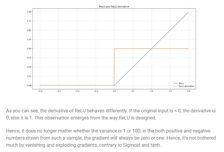
This difference is related to the nonlinearities of the ReLU activation function, which make it non-differentiable at x=0. However at other values it is either 0 or 1 as explained in the image above .The best weight initialization strategy is to initialize the weights randomly but with this variance:

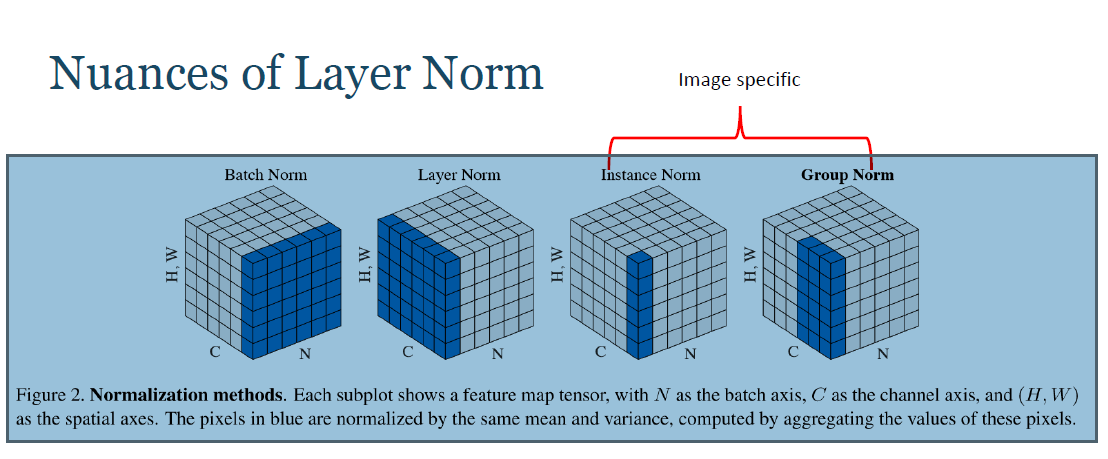
Normalization methods:

Let us recall the meanings of Normalization and standardization in it’s most basic form.

A typical normalization process consists of scaling numerical data down to be on a scale from zero to one, and a typical standardization process consists of subtracting the mean of the dataset from each data point, and then dividing that difference by the data set’s standard deviation.

This forces the standardized data to take on a mean of zero and a standard deviation of one. In practice, this standardization process is often just referred to as normalization as well.

#artificial-neural-network #neural networks