Tutorial on building YOLO v3 detector from scratch detailing how to create the network architecture from a configuration file, load the weights and designing input/output pipelines.

Object detection is a domain that has benefited immensely from the recent developments in deep learning. Recent years have seen people develop many algorithms for object detection, some of which include YOLO, SSD, Mask RCNN and RetinaNet.

For the past few months, I’ve been working on improving object detection at a research lab. One of the biggest takeaways from this experience has been realizing that the best way to go about learning object detection is to implement the algorithms by yourself, from scratch. This is exactly what we’ll do in this tutorial.

We will use PyTorch to implement an object detector based on YOLO v3, one of the faster object detection algorithms out there.

The code for this tutorial is designed to run on Python 3.5, and PyTorch 0.4. It can be found in it’s entirety at this Github repo.

This tutorial is broken into 5 parts:

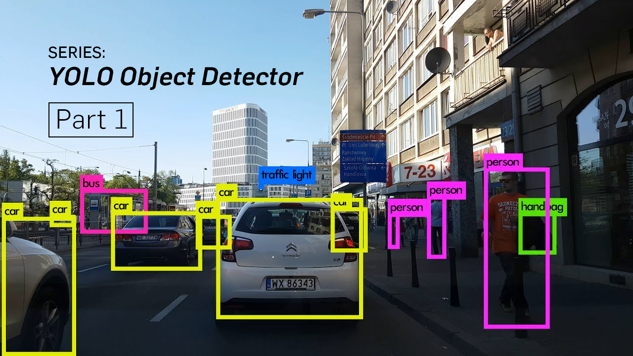
1. Part 1 : Understanding How YOLO works
2. Part 2 : Creating the layers of the network architecture
3. Part 3 : Implementing the the forward pass of the network
4. Part 4 : Confidence Thresholding and Non-maximum Suppression
5. Part 5 : Designing the input and the output pipelines

Prerequisites

• You should understand how convolutional neural networks work. This also includes knowledge of Residual Blocks, skip connections, and Upsampling.
• What is object detection, bounding box regression, IoU and non-maximum suppression.
• Basic PyTorch usage. You should be able to create simple neural networks with ease.

I’ve provided the link at the end of the post in case you fall short on any front.

What is YOLO?

YOLO stands for You Only Look Once. It’s an object detector that uses features learned by a deep convolutional neural network to detect an object. Before we get out hands dirty with code, we must understand how YOLO works.

A Fully Convolutional Neural Network

YOLO makes use of only convolutional layers, making it a fully convolutional network (FCN). It has 75 convolutional layers, with skip connections and upsampling layers. No form of pooling is used, and a convolutional layer with stride 2 is used to downsample the feature maps. This helps in preventing loss of low-level features often attributed to pooling.

Being a FCN, YOLO is invariant to the size of the input image. However, in practice, we might want to stick to a constant input size due to various problems that only show their heads when we are implementing the algorithm.

A big one amongst these problems is that if we want to process our images in batches (images in batches can be processed in parallel by the GPU, leading to speed boosts), we need to have all images of fixed height and width. This is needed to concatenate multiple images into a large batch (concatenating many PyTorch tensors into one)

The network downsamples the image by a factor called the stride of the network. For example, if the stride of the network is 32, then an input image of size 416 x 416 will yield an output of size 13 x 13. Generally, stride of any layer in the network is equal to the factor by which the output of the layer is smaller than the input image to the network.

Interpreting the output

Typically, (as is the case for all object detectors) the features learned by the convolutional layers are passed onto a classifier/regressor which makes the detection prediction (coordinates of the bounding boxes, the class label… etc).

In YOLO, the prediction is done by using a convolutional layer which uses 1 x 1 convolutions.

Now, the first thing to notice is our output is a feature map. Since we have used 1 x 1 convolutions, the size of the prediction map is exactly the size of the feature map before it. In YOLO v3 (and it’s descendants), the way you interpret this prediction map is that each cell can predict a fixed number of bounding boxes.

Though the technically correct term to describe a unit in the feature map would be a neuron, calling it a cell makes it more intuitive in our context.

Depth-wise, we have (B x (5 + C)) entries in the feature map. B represents the number of bounding boxes each cell can predict. According to the paper, each of these B bounding boxes may specialize in detecting a certain kind of object. Each of the bounding boxes have 5 + C attributes, which describe the center coordinates, the dimensions, the objectness score and C class confidences for each bounding box. YOLO v3 predicts 3 bounding boxes for every cell.

You expect each cell of the feature map to predict an object through one of it’s bounding boxes if the center of the object falls in the receptive field of that cell. (Receptive field is the region of the input image visible to the cell. Refer to the link on convolutional neural networks for further clarification).

This has to do with how YOLO is trained, where only one bounding box is responsible for detecting any given object. First, we must ascertain which of the cells this bounding box belongs to.

To do that, we divide the input image into a grid of dimensions equal to that of the final feature map.

Let us consider an example below, where the input image is 416 x 416, and stride of the network is 32. As pointed earlier, the dimensions of the feature map will be 13 x 13. We then divide the input image into 13 x 13 cells.

#pytorch #deep-learning #python #data-science #developer