Python SciPy Tutorial for Beginners with Example

Originally published at https://www.guru99.com

In this Python SciPy Tutorial, you will learn:

What is SciPy?
Why use SciPy
Numpy VS SciPy
SciPy - Installation and Environment Setup
File Input / Output package:
Special Function package:
Linear Algebra with SciPy:
Discrete Fourier Transform – scipy.fftpack
Optimization and Fit in SciPy – scipy.optimize
Nelder –Mead Algorithm:
Image Processing with SciPy – scipy.ndimage

What is SciPy?

SciPy is an Open Source Python-based library, which is used in mathematics, scientific computing, Engineering, and technical computing.

SciPy also pronounced as "Sigh Pi."

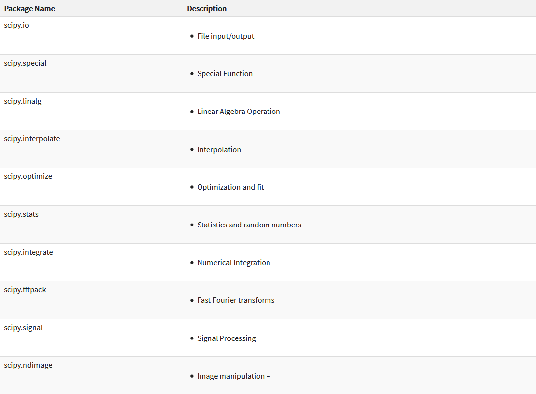
Sub-packages of SciPy:

File input/output - scipy.io
Special Function - scipy.special
Linear Algebra Operation - scipy.linalg
Interpolation - scipy.interpolate
Optimization and fit - scipy.optimize
Statistics and random numbers - scipy.stats
Numerical Integration - scipy.integrate
Fast Fourier transforms - scipy.fftpack
Signal Processing - scipy.signal
Image manipulation – scipy.ndimage

Why use SciPy

SciPy contains varieties of sub packages which help to solve the most common issue related to Scientific Computation.
SciPy is the most used Scientific library only second to GNU Scientific Library for C/C++ or Matlab's.
Easy to use and understand as well as fast computational power.
It can operate on an array of NumPy library.

Numpy VS SciPy

Numpy:

Numpy is written in C and use for mathematical or numeric calculation.
It is faster than other Python Libraries
Numpy is the most useful library for Data Science to perform basic calculations.
Numpy contains nothing but array data type which performs the most basic operation like sorting, shaping, indexing, etc.

SciPy:

SciPy is built in top of the NumPy
SciPy is a fully-featured version of Linear Algebra while Numpy contains only a few features.
Most new Data Science features are available in Scipy rather than Numpy.

SciPy - Installation and Environment Setup

You can also install SciPy in Windows via pip

Python3 -m pip install --user numpy scipy

Install Scipy on Linux

sudo apt-get install  python-scipy python-numpy

Install SciPy in Mac

sudo port install py35-scipy py35-numpy

The standard way of import infSciPy modules and Numpy:

from scipy import special   #same for other modules
import numpy as np

File Input / Output package:

Scipy, I/O package, has a wide range of functions for work with different files format which are Matlab, Arff, Wave, Matrix Market, IDL, NetCDF, TXT, CSV and binary format.

Let's we take one file format example as which are regularly use of MatLab:

 import numpy as np
 from scipy import io as sio
 array = np.ones((4, 4))
 sio.savemat('example.mat', {'ar': array}) 
 data = sio.loadmat(‘example.mat', struct_as_record=True)
 data['array']

Output:

array([[ 1., 1., 1., 1.],
           [ 1., 1., 1., 1.],
           [ 1., 1., 1., 1.],
           [ 1., 1., 1., 1.]])

Code Explanation

Line 1 & 2: Import the essential library scipy with i/o package and Numpy.
Line 3: Create 4 x 4, dimensional one's array
Line 4: Store array in example.mat file.
Line 5: Get data from example.mat file
Line 6: Print output.

Special Function package

scipy.special package contains numerous functions of mathematical physics.
SciPy special function includes Cubic Root, Exponential, Log sum Exponential, Lambert, Permutation and Combinations, Gamma, Bessel, hypergeometric, Kelvin, beta, parabolic cylinder, Relative Error Exponential, etc..
For one line description all of these function, type in Python console:

help(scipy.special)	
Output : 
NAME
    scipy.special
DESCRIPTION

========================================

Special functions (:mod:scipy.special)

========================================
.. module:: scipy.special
 
Nearly all of the functions below are universal functions and follow
broadcasting and automatic array-looping rules. Exceptions are noted.

Cubic Root Function:

Cubic Root function finds the cube root of values.

Syntax:

scipy.special.cbrt(x)

Example:

from scipy.special import cbrt

#Find cubic root of 27 & 64 using cbrt() function

cb = cbrt([27, 64])

#print value of cb

print(cb)

Output: array([3., 4.])

Exponential Function:

Exponential function computes the 10**x element-wise.

Example:

from scipy.special import exp10

#define exp10 function and pass value in its

exp = exp10([1,10])

print(exp)

Output: [1.e+01 1.e+10]

Permutations & Combinations:

SciPy also gives functionality to calculate Permutations and Combinations.

Combinations - scipy.special.comb(N,k)

Example:

from scipy.special import comb

#find combinations of 5, 2 values using comb(N, k)

com = comb(5, 2, exact = False, repetition=True)

print(com)

Output: 15.0

Permutations

scipy.special.perm(N,k)

Example:

from scipy.special import perm

#find permutation of 5, 2 using perm (N, k) function

per = perm(5, 2, exact = True)

print(per)

Output: 20

Log Sum Exponential Function

Log Sum Exponential computes the log of sum exponential input element.

Syntax :

scipy.special.logsumexp(x)

Bessel Function

Nth integer order calculation function

Syntax :

scipy.special.jn()

Linear Algebra with SciPy

Linear Algebra of SciPy is an implementation of BLAS and ATLAS LAPACK libraries.
Performance of Linear Algebra is very fast compared to BLAS and LAPACK.
Linear algebra routine accepts two-dimensional array object and output is also a two-dimensional array.

Now let’s do some test with scipy.linalg,

Calculating determinant of a two-dimensional matrix,

from scipy import linalg

import numpy as np

#define square matrix

two_d_array = np.array([ [4,5], [3,2] ])

#pass values to det() function

linalg.det( two_d_array )

Output: -7.0

Inverse Matrix –

scipy.linalg.inv()

Inverse Matrix of Scipy calculates the inverse of any square matrix.

Let’s see,

from scipy import linalg

import numpy as np
define square matrix
two_d_array = np.array([ [4,5], [3,2] ])

#pass value to function inv()

linalg.inv( two_d_array )

Output:

array( [[-0.28571429,  0.71428571],

[ 0.42857143, -0.57142857]] )

Eigenvalues and Eigenvector – scipy.linalg.eig()

The most common problem in linear algebra is eigenvalues and eigenvector which can be easily solved using eig() function.
Now lets we find the Eigenvalue of (X) and correspond eigenvector of a two-dimensional square matrix.

Example,

from scipy import linalg

import numpy as np

#define two dimensional array

arr = np.array([[5,4],[6,3]])

#pass value into function

eg_val, eg_vect = linalg.eig(arr)

#get eigenvalues

print(eg_val)

#get eigenvectors

print(eg_vect)

Output:

[ 9.+0.j -1.+0.j] #eigenvalues

[ [ 0.70710678 -0.5547002 ] #eigenvectors

[ 0.70710678  0.83205029] ]

Discrete Fourier Transform – scipy.fftpack

DFT is a mathematical technique which is used in converting spatial data into frequency data.
FFT (Fast Fourier Transformation) is an algorithm for computing DFT
FFT is applied to a multidimensional array.
Frequency defines the number of signal or wavelength in particular time period.

Example: Take a wave and show using Matplotlib library. we take simple periodic function example of sin(20 × 2πt)

%matplotlib inline

from matplotlib import pyplot as plt

import numpy as np
#Frequency in terms of Hertz

fre  = 5

#Sample rate

fre_samp = 50

t = np.linspace(0, 2, 2 * fre_samp, endpoint = False )

a = np.sin(fre  * 2 * np.pi * t)

figure, axis = plt.subplots()

axis.plot(t, a)

axis.set_xlabel (‘Time (s)’)

axis.set_ylabel (‘Signal amplitude’)

plt.show()

Output :

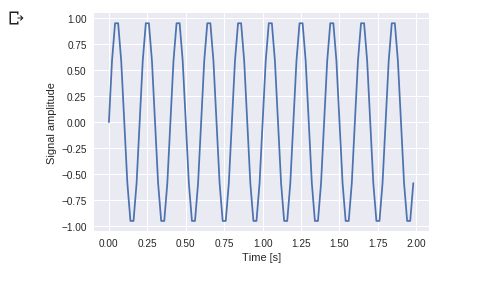
You can see this. Frequency is 5 Hz and its signal repeats in 1/5 seconds – it’s call as a particular time period.

Now let us use this sinusoid wave with the help of DFT application.

from scipy import fftpack
A = fftpack.fft(a)

frequency = fftpack.fftfreq(len(a)) * fre_samp

figure, axis = plt.subplots()
axis.stem(frequency, np.abs(A))

axis.set_xlabel(‘Frequency in Hz’)

axis.set_ylabel(‘Frequency Spectrum Magnitude’)

axis.set_xlim(-fre_samp / 2, fre_samp/ 2)

axis.set_ylim(-5, 110)

plt.show()

Output:

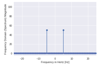
You can clearly see that output is a one-dimensional array.
Input containing complex values are zero except two points.
In DFT example we visualize the magnitude of the signal.

Optimization and Fit in SciPy – scipy.optimize

Optimization provides a useful algorithm for minimization of curve fitting, multidimensional or scalar and root fitting.
Let’s take an example of a Scalar Function, to find minimum scalar function.

%matplotlib inline

import matplotlib.pyplot as plt

from scipy import optimize

import numpy as np
def function(a):

return   a2 + 20 * np.sin(a)

plt.plot(a, function(a))

plt.show()

#use BFGS algorithm for optimization

optimize.fmin_bfgs(function, 0)

Output:

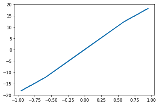
Optimization terminated successfully.

Current function value: -23.241676

Iterations: 4

Function evaluations: 18

Gradient evaluations: 6

array([-1.67096375])

In this example, optimization is done with the help of the gradient descent algorithm from the initial point
But the possible issue is local minima instead of global minima. If we don’t find a neighbor of global minima, then we need to apply global optimization and find global minima function used as basinhopping() which combines local optimizer.

optimize.basinhopping(function, 0)

Output:

fun: -23.241676238045315

lowest_optimization_result:

fun: -23.241676238045315

hess_inv: array([[0.05023331]])

jac: array([4.76837158e-07])

message: ‘Optimization terminated successfully.’

nfev: 15

nit: 3

njev: 5

status: 0

success: True

x: array([-1.67096375])

message: [‘requested number of basinhopping iterations completed successfully’]

minimization_failures: 0

nfev: 1530

nit: 100

njev: 510

x: array([-1.67096375])

Nelder – Mead Algorithm:

Nelder-Mead algorithm selects through method parameter.
It provides the most straightforward way of minimization for fair behaved function.
Nelder – Mead algorithm is not used for gradient evaluations because it may take a longer time to find the solution.

import numpy as np

from scipy.optimize import minimize

#define function f(x)

def f(x):

return .4(1 - x[0])**2
optimize.minimize(f, [2, -1], method=“Nelder-Mead”)

Output:

final_simplex: (array([[ 1.        , -1.27109375],

[ 1.        , -1.27118835],

[ 1.        , -1.27113762]]), array([0., 0., 0.]))

fun: 0.0

message: ‘Optimization terminated successfully.’

nfev: 147

nit: 69

status: 0

success: True

x: array([ 1.        , -1.27109375])

Image Processing with SciPy – scipy.ndimage

scipy.ndimage is a submodule of SciPy which is mostly used for performing an image related operation
ndimage means the “n” dimensional image.
SciPy Image Processing provides Geometrics transformation (rotate, crop, flip), image filtering (sharp and de nosing), display image, image segmentation, classification and features extraction.
MISC Package in SciPy contains prebuilt images which can be used to perform image manipulation task

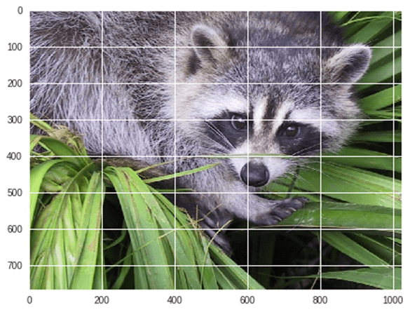
Example: Let’s take a geometric transformation example of images

from scipy import misc

from matplotlib import pyplot as plt

import numpy as np

#get face image of panda from misc package

panda = misc.face()

#plot or show image of face

plt.imshow( panda )

plt.show()

Output:

Now we Flip-down current image:

#Flip Down using scipy misc.face image

flip_down = np.flipud(misc.face())

plt.imshow(flip_down)

plt.show()

Output:

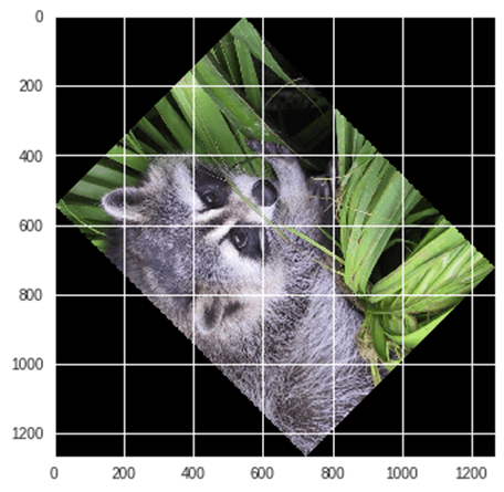
Example: Rotation of Image using Scipy,

from scipy import ndimage, misc

from matplotlib import pyplot as plt

panda = misc.face()

#rotatation function of scipy for image – image rotated 135 degree

panda_rotate = ndimage.rotate(panda, 135)

plt.imshow(panda_rotate)

plt.show()

Output:

Integration with Scipy – Numerical Integration

When we integrate any function where analytically integrate is not possible, we need to turn for numerical integration
SciPy provides functionality to integrate function with numerical integration.
scipy.integrate library has single integration, double, triple, multiple, Gaussian quadrate, Romberg, Trapezoidal and Simpson’s rules.

Example: Now take an example of Single Integration

Here a is the upper limit and b is the lower limit

from scipy import integrate
take f(x) function as f
f = lambda x : x**2

#single integration with a = 0 & b = 1

integration = integrate.quad(f, 0 , 1)

print(integration)

Output:

(0.33333333333333337, 3.700743415417189e-15)

Here function returns two values, in which the first value is integration and second value is estimated error in integral.

Example: Now take an example of double integration. We find the double integration of the following equation,

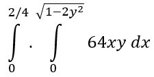
from scipy import integrate

import numpy as np

#import square root function from math lib

from math import sqrt
set  fuction f(x)
f = lambda x, y : 64 xy
lower limit of second integral
p = lambda x : 0
upper limit of first integral
q = lambda y : sqrt(1 - 2*y**2)
perform double integration
integration = integrate.dblquad(f , 0 , 2/4,  p, q)

print(integration)

Output:

(3.0, 9.657432734515774e-14)

You have seen that above output as same previous one.

Summary

SciPy(pronounced as “Sigh Pi”) is an Open Source Python-based library, which is used in mathematics, scientific computing, Engineering, and technical computing.
SciPy contains varieties of sub packages which help to solve the most common issue related to Scientific Computation.
SciPy is built in top of the NumPy

Thanks for reading ❤

If you liked this post, share it with all of your programming buddies!

Python SciPy Tutorial for Beginners with Example

What is SciPy?

Why use SciPy

Numpy VS SciPy

SciPy - Installation and Environment Setup

File Input / Output package:

Special Function package

Cubic Root Function:

Exponential Function:

Permutations & Combinations:

Log Sum Exponential Function

Bessel Function

Linear Algebra with SciPy

define square matrix

Discrete Fourier Transform – scipy.fftpack

Optimization and Fit in SciPy – scipy.optimize

Nelder – Mead Algorithm:

Image Processing with SciPy – scipy.ndimage

Integration with Scipy – Numerical Integration

take f(x) function as f

set fuction f(x)

lower limit of second integral

upper limit of first integral

perform double integration

Summary

Further reading