In Part 1 of our series on how to write efficient code using NumPy, we covered the important topics of vectorization and broadcasting. In this part we will put these concepts into practice by implementing an efficient version of the K-Means clustering algorithm using NumPy. We will benchmark it against a naive version implemented entirely using looping in Python. In the end we’ll see that the NumPy version is about 70 times faster than the simple loop version.
To be exact, in this post we will cover:
- Understanding K-Means Clustering
- Implementing K-Means using loops
- Using cProfile to find bottlenecks in the code
- Optimizing K-Means using NumPy
Let’s get started!
Understanding K-Means Clustering
In this post we will be optimizing an implementation of the k-means clustering algorithm. It is therefore imperative that we at least have a basic understanding of how the algorithm works. Of course, a detailed discussion would also be beyond the scope of this post; if you want to dig deeper into k-means you can find several recommended links below.
What Does the K-Means Clustering Algorithm Do?
In a nutshell, k-means is an unsupervised learning algorithm which separates data into groups based on similarity. As it’s an unsupervised algorithm, this means we have no labels for the data.
The most important hyperparameter for the k-means algorithm is the number of clusters, or k. Once we have decided upon our value for k, the algorithm works as follows.
- Initialize k points (corresponding to k clusters) randomly from the data. We call these points centroids.
- For each data point, measure the L2 distance from the centroid. Assign each data point to the centroid for which it has the shortest distance. In other words, assign the closest centroid to each data point.
- Now each data point assigned to a centroid forms an individual cluster. For k centroids, we will have k clusters. Update the value of the centroid of each cluster by the mean of all the data points present in that particular cluster.
- Repeat steps 1-3 until the maximum change in centroids for each iteration falls below a threshold value, or the clustering error converges.
Here’s the pseudo-code for the algorithm.
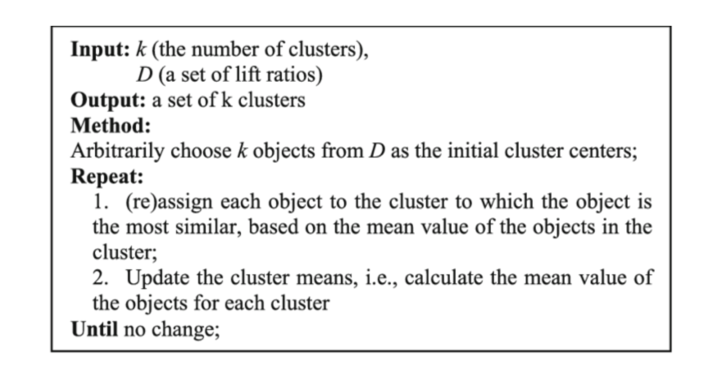 Pseudo-code for the K-Means Clustering Algorithm
I’m going to leave K-Means at that. This is enough to help us code the algorithm. However, there is much more to it, such as how to choose a good value of k, how to evaluate the performance, which distance metrics can be used, preprocessing steps, and theory. In case you wish to dig deeper, here are a few links for you to study it further.
Now, let’s proceed with the implementation of the algorithm.
Implementing K-Means Using Loops
In this section we will be implementing the K-Means algorithm using Python and loops. We will not be using NumPy for this. This code will be used as a benchmark for our optimized version.
Generating the Data
To perform clustering, we first need our data. While we can choose from multiple datasets online, let’s keep things rather simple and intuitive. We are going to synthesize a dataset by sampling from multiple Gaussian distributions, so that visualizing clusters is easy for us.
In case you don’t know what a Gaussian distribution is, check it out!
We will create data from four Gaussian’s with different means and distributions.
import numpy as np
## Size of dataset to be generated. The final size is 4 * data_size
data_size = 1000
num_iters = 50
num_clusters = 4

## sample from Gaussians
data1 = np.random.normal((5,5,5), (4, 4, 4), (data_size,3))
data2 = np.random.normal((4,20,20), (3,3,3), (data_size, 3))
data3 = np.random.normal((25, 20, 5), (5, 5, 5), (data_size,3))
data4 = np.random.normal((30, 30, 30), (5, 5, 5), (data_size,3))

## Combine the data to create the final dataset
data = np.concatenate((data1,data2, data3, data4), axis = 0)

## Shuffle the data
np.random.shuffle(data)
In order to aid our visualization, let’s plot this data in a 3-D space.
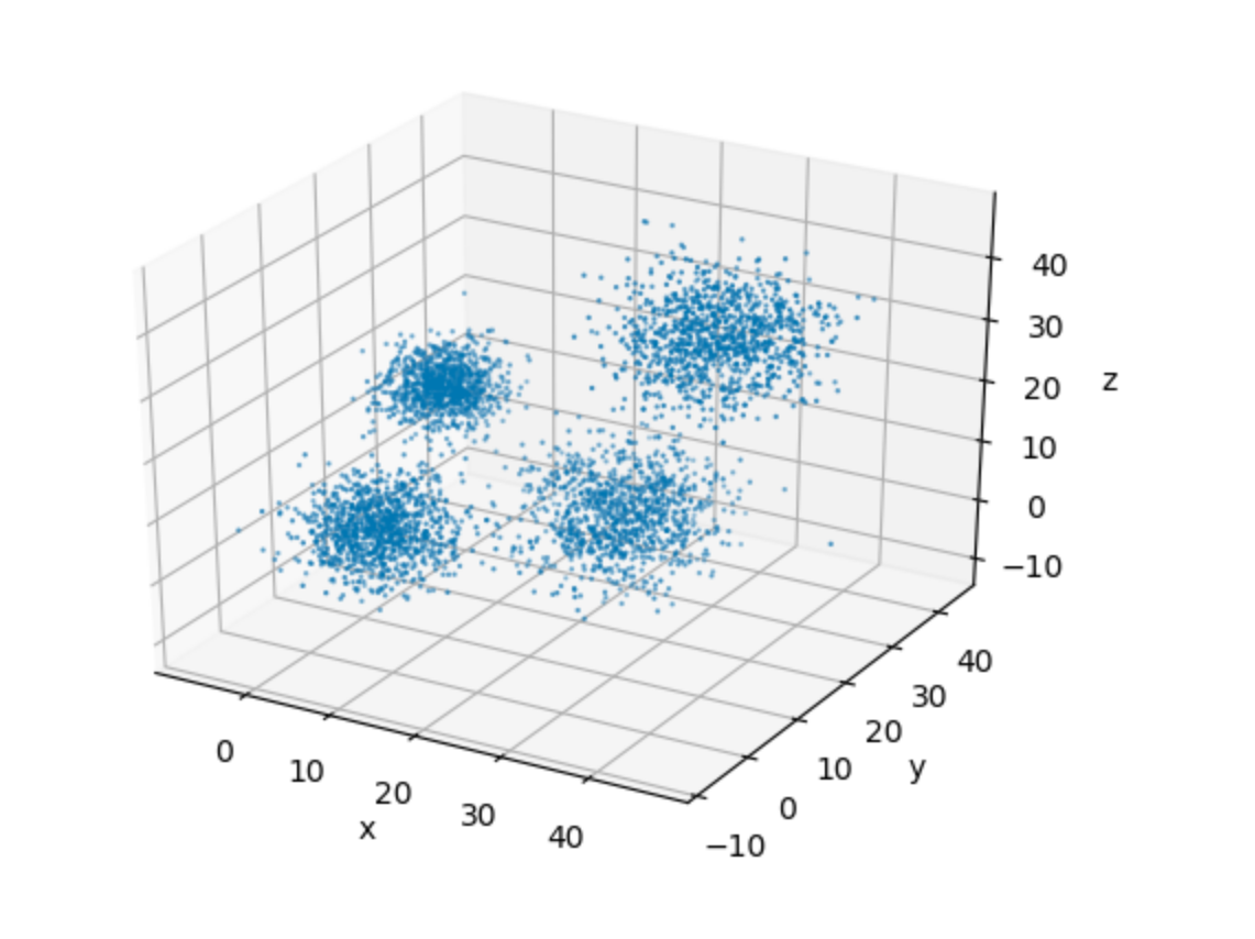 3-D Visualization of the Dataset
It’s very easy to see the four clusters of data in the plot above. This, for one, makes it easy for us to pick up a suitable value of k for our implementation. This goes in spirit of keeping the algorithmic details as simple as possible, so that we can focus on the implementation.
Helper Functions
We begin by initializing our centroids, as well as a list to keep track of which centroid each data point is assigned to.
## Set random seed for reproducibility
random.seed(0)

## Initialize the list to store centroids
centroids = []

## Sample initial centroids
random_indices = random.sample(range(data.shape[0]), 4)
for i in random_indices:
    centroids.append(data[i])

## Create a list to store which centroid is assigned to each dataset
assigned_centroids = [0] * len(data)
Before we implement our loop, we will first implement a few helper functions.
compute_l2_distance takes two points (say [0, 1, 0] and [4, 2, 3]) and computes the L2 distance between them, according to the following formula.
L2(X1,X2)=∑dimensions(X1)i(X1[i]−X2[i])2
L2(X1,X2)=i∑dimensions(X1)(X1[i]−X2[i])2
def compute_l2_distance(x, centroid):
    ## Initialize the distance to 0
    dist = 0

    ## Loop over the dimensions. Take squared difference and add to 'dist'
    for i in range(len(x)):
        dist += (centroid[i] - x[i])**2

    return dist
The other helper function we implement is called get_closest_centroid, the name being pretty self-explanatory. The function takes an input x and a list, centroids, and returns the index of the list centroids corresponding to the centroid closest to x.
def get_closest_centroid(x, centroids):
    ## Initialize the list to keep distances from each centroid
    centroid_distances = []

    ## Loop over each centroid and compute the distance from data point.
    for centroid in centroids:
        dist = compute_l2_distance(x, centroid)
        centroid_distances.append(dist)

    ## Get the index of the centroid with the smallest distance to the data point
    closest_centroid_index =  min(range(len(centroid_distances)), key=lambda x: centroid_distances[x])

    return closest_centroid_index
Then we implement the function compute_sse, which computes the SSE or Sum of Squared Errors. This metric is used to guide how many iterations we have to do. Once this value converges, we can stop training.
def compute_sse(data, centroids, assigned_centroids):
    ## Initialise SSE
    sse = 0

    ## Compute the squared distance for each data point and add.
    for i,x in enumerate(data):
    	## Get the associated centroid for data point
        centroid = centroids[assigned_centroids[i]]

        ## Compute the distance to the centroid
        dist = compute_l2_distance(x, centroid)

        ## Add to the total distance
        sse += dist

    sse /= len(data)
    return sse
Main Loop
Now, let’s write the main loop. Refer to the pseudo-code mentioned above for reference. Instead of looping until convergence, we merely loop for 50 iterations.
## Number of dimensions in centroid
num_centroid_dims = data.shape[1]

## List to store SSE for each iteration
sse_list = []

tic = time.time()

## Loop over iterations
for n in range(num_iters):

    ## Loop over each data point
    for i in range(len(data)):
        x = data[i]

        ## Get the closest centroid
        closest_centroid = get_closest_centroid(x, centroids)

        ## Assign the centroid to the data point.
        assigned_centroids[i] = closest_centroid

    ## Loop over centroids and compute the new ones.
    for c in range(len(centroids)):
        ## Get all the data points belonging to a particular cluster
        cluster_data = [data[i] for i in range(len(data)) if assigned_centroids[i] == c]

        ## Initialize the list to hold the new centroid
        new_centroid = [0] * len(centroids[0])

        ## Compute the average of cluster members to compute new centroid
        ## Loop over dimensions of data
        for dim in range(num_centroid_dims):
            dim_sum = [x[dim] for x in cluster_data]
            dim_sum = sum(dim_sum) / len(dim_sum)
            new_centroid[dim] = dim_sum

        ## assign the new centroid
        centroids[c] = new_centroid

    ## Compute the SSE for the iteration
    sse = compute_sse(data, centroids, assigned_centroids)
    sse_list.append(sse)
The entire code can be viewed below.
import numpy as np
import matplotlib.pyplot as plt
import random
import time

## Size of dataset to be generated. The final size is 4 * data_size
data_size = 1000
num_iters = 50
num_clusters = 4

## sample from Gaussians
data1 = np.random.normal((5,5,5), (4, 4, 4), (data_size,3))
data2 = np.random.normal((4,20,20), (3,3,3), (data_size, 3))
data3 = np.random.normal((25, 20, 5), (5, 5, 5), (data_size,3))
data4 = np.random.normal((30, 30, 30), (5, 5, 5), (data_size,3))

## Combine the data to create the final dataset
data = np.concatenate((data1,data2, data3, data4), axis = 0)

## Shuffle the data
np.random.shuffle(data)

## Set random seed for reproducibility
random.seed(0)

## Initialise the list to store centroids
centroids = []

## Sample initial centroids
random_indices = random.sample(range(data.shape[0]), 4)
for i in random_indices:
    centroids.append(data[i])

## Create a list to store which centroid is assigned to each dataset
assigned_centroids = [0] * len(data)

def compute_l2_distance(x, centroid):
    ## Initialise the distance to 0
    dist = 0

    ## Loop over the dimensions. Take sqaured difference and add to `dist`
    for i in range(len(x)):
        dist += (centroid[i] - x[i])**2

    return dist

def get_closest_centroid(x, centroids):
    ## Initialise the list to keep distances from each centroid
    centroid_distances = []

    ## Loop over each centroid and compute the distance from data point.
    for centroid in centroids:
        dist = compute_l2_distance(x, centroid)
        centroid_distances.append(dist)

    ## Get the index of the centroid with the smallest distance to the data point
    closest_centroid_index =  min(range(len(centroid_distances)), key=lambda x: centroid_distances[x])

    return closest_centroid_index

def compute_sse(data, centroids, assigned_centroids):
    ## Initialise SSE
    sse = 0

    ## Compute the squared distance for each data point and add.
    for i,x in enumerate(data):
    	## Get the associated centroid for data point
        centroid = centroids[assigned_centroids[i]]

        ## Compute the Distance to the centroid
        dist = compute_l2_distance(x, centroid)

        ## Add to the total distance
        sse += dist

    sse /= len(data)
    return sse

## Number of dimensions in centroid
num_centroid_dims = data.shape[1]

## List to store SSE for each iteration
sse_list = []

tic = time.time()

## Loop over iterations
for n in range(num_iters):

    ## Loop over each data point
    for i in range(len(data)):
        x = data[i]

        ## Get the closest centroid
        closest_centroid = get_closest_centroid(x, centroids)

        ## Assign the centroid to the data point.
        assigned_centroids[i] = closest_centroid

    ## Loop over centroids and compute the new ones.
    for c in range(len(centroids)):
        ## Get all the data points belonging to a particular cluster
        cluster_data = [data[i] for i in range(len(data)) if assigned_centroids[i] == c]

        ## Initialise the list to hold the new centroid
        new_centroid = [0] * len(centroids[0])

        ## Compute the average of cluster members to compute new centroid
        ## Loop over dimensions of data
        for dim in range(num_centroid_dims):
            dim_sum = [x[dim] for x in cluster_data]
            dim_sum = sum(dim_sum) / len(dim_sum)
            new_centroid[dim] = dim_sum

        ## assign the new centroid
        centroids[c] = new_centroid

    ## Compute the SSE for the iteration
    sse = compute_sse(data, centroids, assigned_centroids)
    sse_list.append(sse)

#
toc = time.time()
print((toc - tic)/50)
#numpy #python #machine-learning #data-science #dveloper